Writing reproducible, re-usable reports, with R + markdown
Peter Ralph
September 29, 2020
Markdown
Goal:
Communicate your thoughts to your collaborators and your future self,
combining text, math, documented code,
and no fuss.
No fussing about layout:
Markdown aims to be readable as-is,
but has methods to produce beautiful output.
A Markdown-formatted document should be publishable as-is, as plain text, without looking like it’s been marked up with tags or formatting instructions. – John Gruber
No, really, don’t think about the layout
Don’t even think about the layout, just the content.
[…] it is better to leave document design to document designers, and to let authors get on with writing documents – intro to LaTeX
Today’s goal:
- Learn a few simple rules
- and get going producing content.
Structuring text
- Separate things with empty lines.
- Wrap lines whenever you feel like it.
Source
Result
Text formatting
Inline markup
Paragraphs begin and end with empty lines, and are not indented.
- bold and emphasis
strikeout- superscripts and subscripts
- and
inline_code($fixed.width)
Source
Lists must be preceded by an empty line,
- ordered or unordered.
Indenting subsequent content
will continue the list
- and nest
- other lists.
Indenting means one tab, or four spaces.
After using markdown for a bit, go read pandoc’s documentation.
Math
Math goes between `$`, single ($\pi$), or double:
$$ \frac{\pi}{4} = \sum_{n=0}^\infty \frac{(-1)^n}{2k+1} .$$
Math goes between $, single (\(\pi\)), or double: \[\frac{\pi}{4} = \sum_{n=0}^\infty \frac{(-1)^n}{2k+1} .\]
Even math environments inside double dollar signs:
\[\begin{align} x &= (a+b)^2 - (a-b)^2 \\ &= 4ab \end{align}\]
Code blocks
```{.r}
msg <- "Hello, world."
print(msg)
```
produces
Blockquotes
> I also dream about a modern replacement for LaTeX
> designed from the ground up to target multiple output formats
> (at least PDF, HTML, EPUB). -- [John MacFarlane](http://john.macfarlane.usesthis.com/)
produces
I also dream about a modern replacement for LaTeX designed from the ground up to target multiple output formats (at least PDF, HTML, EPUB). – John MacFarlane
Links and Images
Images are the same but with a ! in front.
Setting width and height are optional.

Rendering markdown with pandoc
Get started!
Directions / in Rstudio.
- Make a directory for this workshop
/ start a new project. - Open a text editor
/ open a new Rmarkdown file and delete everything. - Write some text.
- Save it as
notes.Rmd.
To compile, either:
Open
R, runand open
notes.htmlin your web browser.or in
Rstudio, save the file (with suffix.Rmd) and click on knit.
Where is it? Use getwd() to tell you.
Wait, but the layout?
Remember,
[…] it is better to leave document design to document designers, and to let authors get on with writing documents.
If you must, then:
- tweak the css
- modify a rmarkdown format
- or a pandoc template
Gotchas
- many things need to begin with an empty line
- carriage returns don’t (usually) mean anything
- but indentations do (by at least four spaces)
For more info see the documentation.
Metadata
At the top of your document, add
… the YAML metadata,
delimited by exactly three dashes.
Note: Besides setting the title, you can control the output in many ways here.
For example: add
and render with rmarkdown::render("notes.md").
or even:
Under the hood
Adding in R
Goal: add R code to the document, along with its output.

Go ahead
Just add a chunk of R code, wrapped in
 ```{r}
 # PUT ARBITRARY R CODE HERE
 ```
Try it!
Powers of two?

 ```{r}
 2^(0:10)
```How about this?
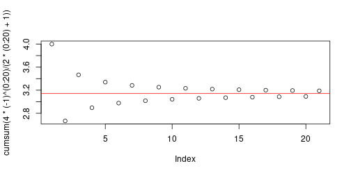
$$ \lim_{n \to \infty} 4 \sum_{k=1}^n \frac{ (-1)^n }{ 2n+1 } = \pi , $$
```{r}
cumsum( 4 * (-1)^(0:20) / (2*(0:20)+1) )
```How about this? \[ \lim_{n \to \infty} 4 \sum_{k=0}^n \frac{ (-1)^n }{ 2n+1 } = \pi , \]
## [1] 4.000000 2.666667 3.466667 2.895238 3.339683 2.976046 3.283738 3.017072 3.252366 3.041840 3.232316 3.058403 3.218403 3.070255 3.208186 3.079153 3.200366 3.086080 3.194188 3.091624 3.189185 ```{r}
plot(cumsum( 4 * (-1)^(0:20) / (2*(0:20)+1) ))
abline(h=pi, col='red')
```
Exercise
Make a short Rmarkdown document that
checks that \[1 + 2 + \cdots + n = n(n+1)/2\] for every \(n\) between 1 and 100
shows these on a plot
explains what’s being computed
Useful: x = cumsum(1:100) and plot(x) and lines(y).
What’s going on
knitruses a regular expression to find code chunks- pulls these out,
- evaluates them one at a time
- and inserts “the results” back in
pandocrenders the resulting markdown file- with various choices of styling
Chunk options
Name each chunk, and set options for what gets printed
```{r my_chunk_name, fig.height=4, echo=FALSE}echo=(TRUE|FALSE)include source code in the output?
results="(markup|asis)"style the output or not?
include=(FALSE|TRUE)include anything in the output?
Set document defaults up top:
 ```{r, include=FALSE}
 fig.dim <- 5
 library(knitr)
 opts_chunk$set(
        fig.height=fig.dim,
        fig.width=2*fig.dim,
        fig.align='center'
    )
 ```
Tables
One option: use pander.
 ```{r}
 library(pander)
 bases <- table( sample( c("A","C","G","T"), 300, replace=TRUE ) )
 pander(t(bases))
 ```
note: the transpose t( )
| A | C | G | T |
|---|---|---|---|
| 70 | 85 | 83 | 62 |
Inline code
You can
`r paste(letters[c(9,14,19,5,18,20)],collapse='')`
code anywhere.
You can insert code anywhere.
Even in the YAML header.
Go change yours!
---
title: "My notes"
author: "Peter Ralph"
date: "`r date()`"
---
Online example
Goal: Write a function that will generate all sequences of A/C/G/T of length \(n\) for which no two adjacent letters are the same.
Here is a pre-written solution.
Your turn
Download the iris dataset to a new directory.
or just do
Read in the data.
Describe the dataset: number of observations, variables, etcetera.
- inline
Rcode (`r nrow(iris)`)
- inline
Make a table of the number of observations for each species.
pander()- or
results="asis"andprint.xtable(xtable( ),type='html')
Plot the flower dimensions against each other,
- using
pairs(), and colored by species.
- using
Templated reports
Set up some fake data: each has 50 observations of two quantitative variables (age and height) and a categorical variable (type):
dir.create("examples/thedata")
owd <- setwd("examples/thedata")
for (samp in LETTERS[1:8]) {
    dir.create(samp)
    xy <- data.frame(
        age=exp(rnorm(50)),
        type=sample(letters[1:3],50,replace=TRUE)
    )
    xy$height <- 5 + runif(1)*xy$age + 3*runif(1)*as.numeric(xy$type) + rnorm(50)
    write.table(xy,file=paste0(samp,"/data.tsv"))
}
setwd(owd)
We now have 10 datasets, each in a file like A/data.tsv. Here’s what one looks like:
## age type height
## 1 1.4796488 c 9.361211
## 2 1.0046351 b 7.809438
## 3 0.8169789 c 8.509819
## 4 0.1572326 a 5.702507
## 5 0.2543326 a 6.924387
## 6 8.1443866 b 13.790307
## 7 0.8223393 a 7.054007
## 8 6.1442730 b 13.426498
## 9 3.0191242 b 9.207488
## 10 0.7728761 c 7.260055
## 11 2.7337382 a 8.775505
## 12 4.9572850 b 10.785370
## 13 1.1893305 b 7.997365
## 14 7.4601762 a 11.033910
## 15 0.2412250 b 5.188430
## 16 1.7532513 c 9.365491
## 17 0.5922570 c 7.953115
## 18 1.1926213 b 10.210615
## 19 1.0236192 b 6.526443
## 20 5.1199085 b 8.518106
## 21 0.9541798 a 5.253971
## 22 0.3123665 b 5.506721
## 23 1.0759528 a 5.045323
## 24 1.4650504 a 6.649536
## 25 1.6650421 a 7.217283
## 26 1.1198742 b 6.362583
## 27 1.2415980 b 7.193038
## 28 2.4319417 b 8.180893
## 29 0.5862522 b 6.385537
## 30 0.8680723 b 7.183052
## 31 0.6600719 b 6.006921
## 32 0.7879503 b 6.422339
## 33 2.5323571 c 9.426129
## 34 0.2440238 c 7.841699
## 35 0.7925729 a 5.619829
## 36 3.0982004 c 9.460839
## 37 1.2647280 b 6.505928
## 38 2.3627868 a 8.699527
## 39 0.4884444 a 5.547974
## 40 0.4585299 a 6.704829
## 41 0.3537712 c 7.097977
## 42 3.4127451 b 8.615107
## 43 0.7935832 a 6.186167
## 44 0.5354499 c 6.376454
## 45 1.0126319 c 6.952713
## 46 0.3659778 c 6.663840
## 47 0.9081240 c 8.437199
## 48 0.4860253 b 6.594441
## 49 0.3530557 a 7.768926
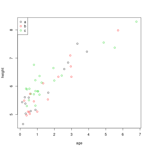
## 50 0.5318298 a 5.175261We would like to visualize each, like this:
The template: examples/simple-template.Rmd
 ---
 title: "Visualization for `r getwd()`"
 date: "`r date()`"
 ---

 ```{r setup, echo=FALSE}
 input.file <- "data.tsv"
 xy <- read.table(input.file)
 ```

 The file `r normalizePath(input.file)`
 has `r nrow(xy)` observations:

 ```{r}
 plot( height ~ age, col=type, data=xy )
 legend( "topleft", pch=1, col=1:nlevels(xy$type) )
 ```
Input: this looks for the file data.tsv in the current directory.
Render it:
Option 1: copy the template into each of the ten directories, and render them there.
Option 2: use my templater package.
library(devtools)
install_github("petrelharp/templater")
library(templater)
dir.names <- file.path("examples/thedata", LETTERS[1:8])
for (input.dir in dir.names) {
    output.file <- file.path(input.dir, "visualization.html")
    render_template("examples/simple-template.Rmd", output=output.file,
                    change.rootdir=TRUE, quiet=TRUE)
}
Look at them:
 ```{r make_links, results="asis"}
 output.files <- file.path("examples/thedata", LETTERS[1:8], "visualization.html")
 links <- paste("[",dir.names,"](",output.files,")",sep='')
 cat( paste("- ", links, "\n"), "\n" )
```Another exercise
Goal: Compare different \(k\) with \(k\)-means on the iris dataset.
- Make subdirectories, called
iris/k, for \(1 \le k \le 5\), - and in each runs
kmeanswith the appropriatek.
Example:
Other resources
- Karl Broman’s intro to Rmarkdown
- the extensive, excellent documentation for pandoc
- StackOverflow
- my technical notes I made while writing this up