New tools for popgen simulation and analysis:
What’s possible?
Evolution 2021
slides: github:petrelharp/evolution_2021
Overview of simulators
In this talk:
Forwards or backwards?

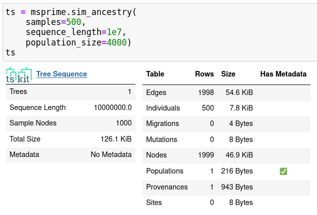
msprime
msprime v1.0
New features:
- \(k\)-ploid individuals, finite sites
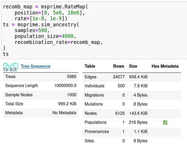
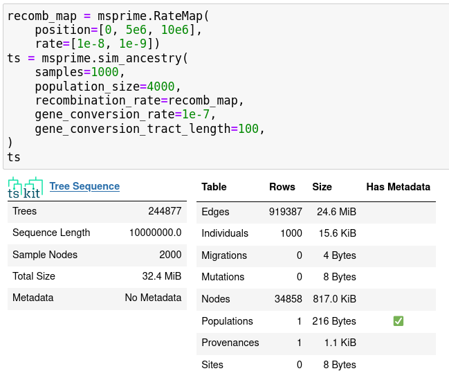
- recombination rate maps
- gene conversion
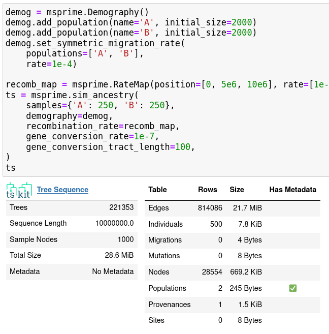
- nicer demographic model specification
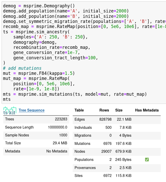
- mutation rate maps
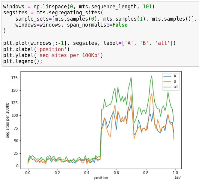
- quick analysis
New features:
- \(k\)-ploid individuals, finite sites
- recombination rate maps
- gene conversion
- nicer demographic model specification
- mutation rate maps
- quick analysis
New features:
- \(k\)-ploid individuals, finite sites
- recombination rate maps
- gene conversion
- nicer demographic model specification
- mutation rate maps
- quick analysis
New features:
- \(k\)-ploid individuals, finite sites
- recombination rate maps
- gene conversion
- nicer demographic model specification
- mutation rate maps
- quick analysis
New features:
- \(k\)-ploid individuals, finite sites
- recombination rate maps
- gene conversion
- nicer demographic model specification
- mutation rate maps
- quick analysis
New features:
- \(k\)-ploid individuals, finite sites
- recombination rate maps
- gene conversion
- nicer demographic model specification
- mutation rate maps
- quick analysis
Ancestry models
- “the” coalescent
- discrete-time Wright-Fisher
- multiple mergers
- selective sweeps
sweep_model = msprime.SweepGenicSelection(
    position=2.5e4, s=0.01,
    start_frequency=0.5e-4, end_frequency=0.99, dt=1e-6)
sts = msprime.sim_ancestry(9,
    model=[sweep_model, msprime.StandardCoalescent()],
    population_size=1e4, recombination_rate=1e-8, sequence_length=5e4)
Mutation models
- infinite sites/alleles
- nucleotides
- amino acids
- arbitrary Markovian models
dem = msprime.Demography.from_species_tree(
   "((A:900,B:900)ab:100,C:1000)abc;",
   initial_size=1e3)
samples = {"A": 2, "B": 1, "C": 1}
ts = msprime.sim_ancestry(
   8, demography=dem, sequence_length=5e4,
   recombination_rate=1e-8
)
mts = msprime.sim_mutations(ts, rate=1e-7)
mts.draw_svg()
An eco-evolutionary simulator
- everything msprime can
- ecological dynamics with “non-Wright-Fisher” models
- populations in continuous, heterogeneous geography
- sex chromosomes, haplodiploidy
- complex traits
- context-dependent mutations
- v4: interacting species

Ben Haller
tree sequences
Development philosophy
- open, welcoming, supportive
- well-documented
- reliable, reproducible
- backwards compatible
Benefits

Post-hoc mutations

Recapitation

msprime: 1000 samples
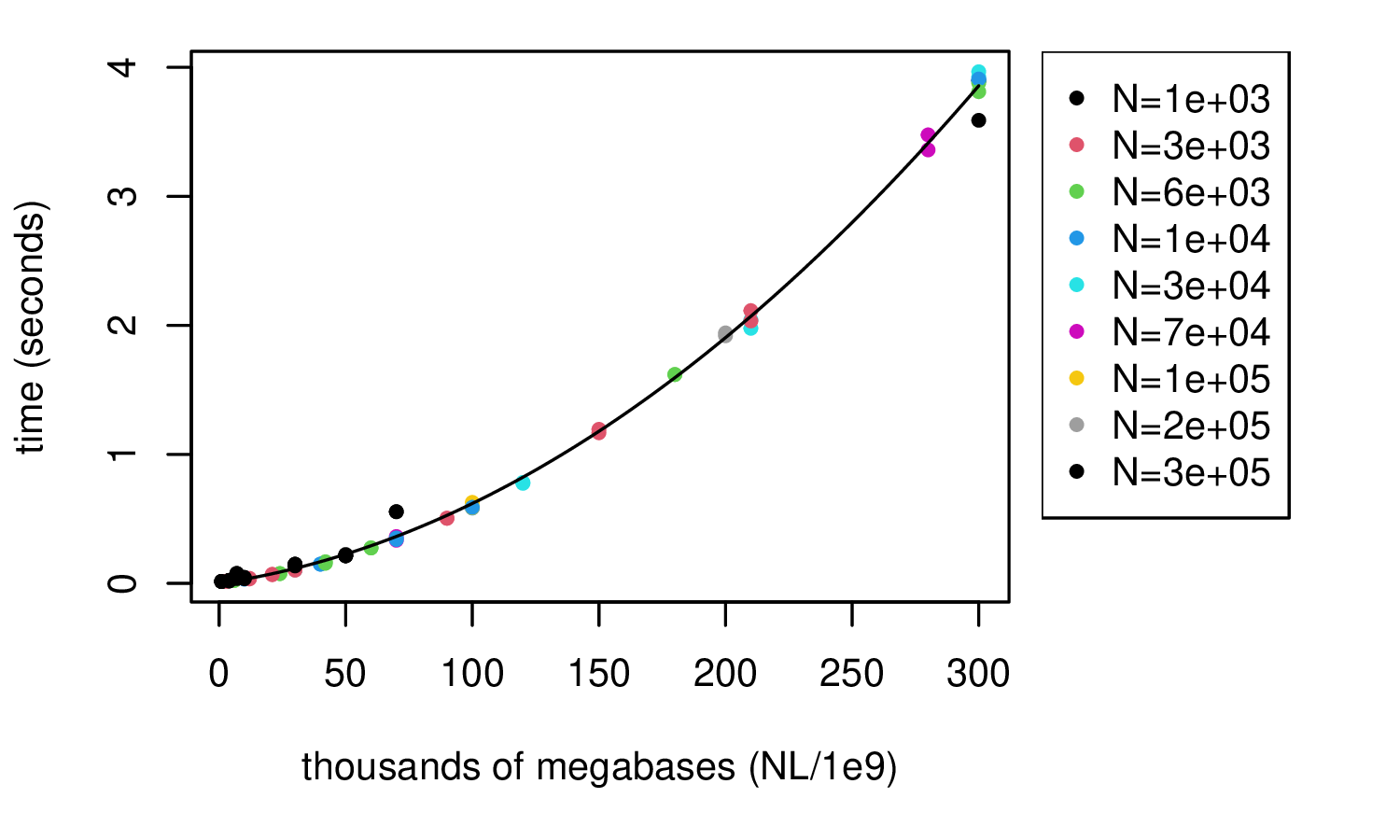
takeaway: hundreds of thousands of megabases takes seconds
msprime: 1000 samples
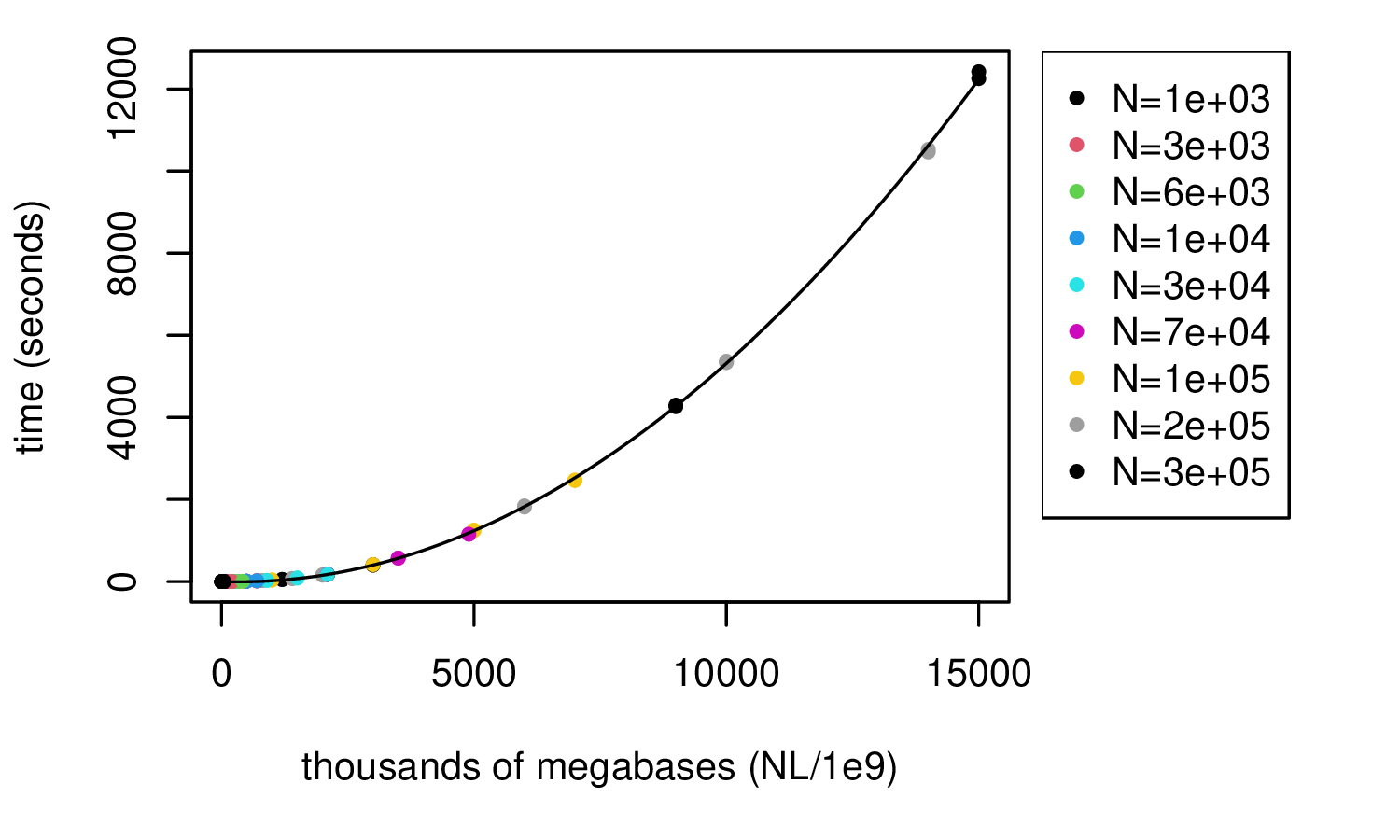
takeaway: hundreds of thousands of megabases takes seconds
basic demography: SLiM
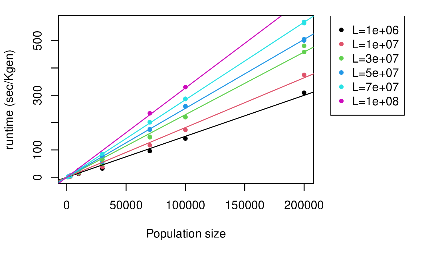
takeaway: linear in population size
Basic demography: SLiM
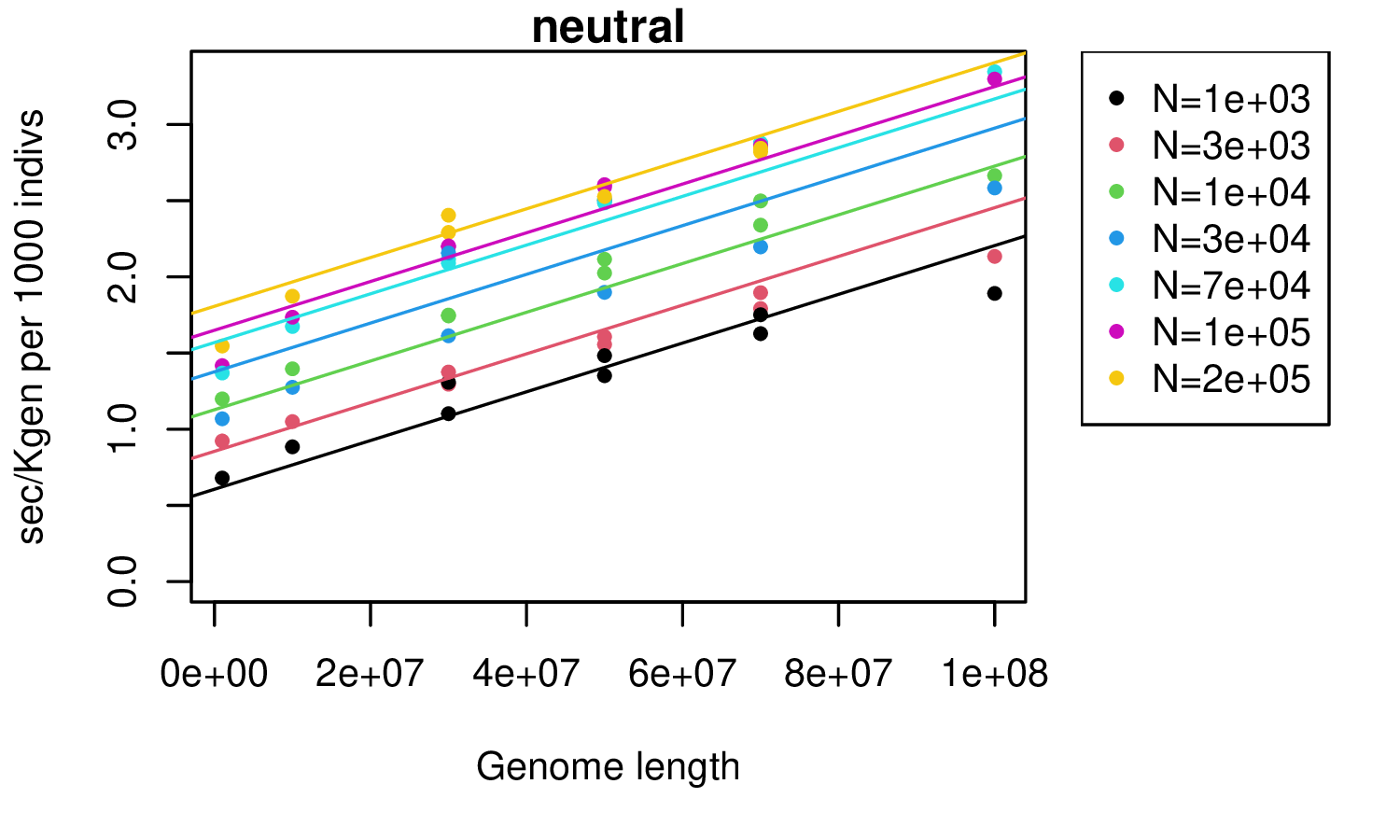
takeaway: seconds per thousand individuals per thousand generations
Selection: SLiM, total rate \(10^{-10}\)
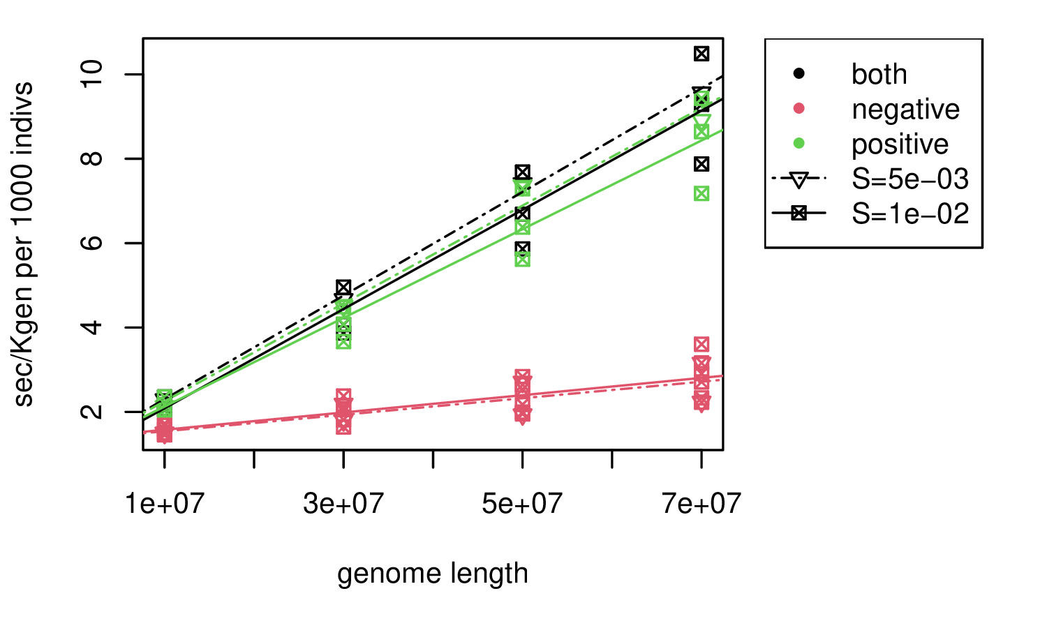
takeaway: similar, but slower by a factor of 3 for lots of positive mutations
Spatial simulations: SLiM
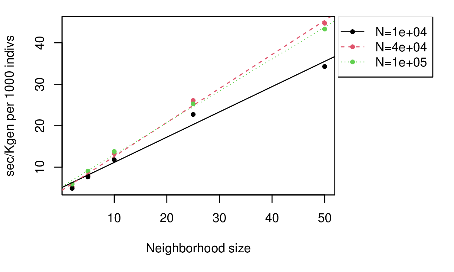
takeaway: 3x slower than genomes! Scales with neighborhood size (\(\sigma^2\)).
Thanks!


- Jerome Kelleher
- Ben Haller
- Ben Jeffery
- Yan Wong
- Murillo Rodrigues
- Andy Kern
- Philipp Messer