Poisson Point Processes

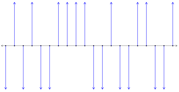
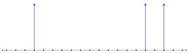
Matt Lukac email: mlukac@uoregon.edu

December 27, 2018

Recall a realization of the basic noise for Gaussian processes looked like that in Figure 1. Now, arrows are either muted or (rarely) point up. See Figure 2.

Figure 1: A realization of the basic noise used to construct a Gaussian process.

Figure 2: A realization of the basic noise used to construct a Poisson process.

1 Motivation

Suppose in some space $X$ we lay down a large number of LED lights, each with their own battery, with density given by a $\sigma$ -finite measure $\mu$ . We do this in a way so that, for each region $A\subset X$ , we put down about $M\mu(A)$ lights in that region, where $M$ is some large number. Independently we turn on each light with probability $M^{-1}$ , and leave off otherwise.

We would like to answer the following question: how many lights in $A$ are on? To that end, let $N(A)$ denote the number of lights on in $A$ and compute

\displaystyle\mathbb{E}\left[N(A)\right]=\mathbb{E}\left[\sum_{\text{lights in% }A}\mathds{1}_{\{\text{light on}\}}\right]=\sum_{\text{lights in }A}\mathbb{P% }\left\{\text{light is on}\right\}=M\mu(A)\left(\frac{1}{M}\right)=\mu(A).

(1)

Thus $\mu$ gives the expected density for the set of lights that are on in $A$ . By construction, we know $N(A)\sim\operatorname{Binom}\left(M\mu(A),M^{-1}\right)$ , and hence the distribution of $N(A)$ is approximately $\operatorname{Pois}(\mu(A))$ . To see this, put $L=M\mu(A)$ and observe,

$\displaystyle\mathbb{P}\left\{N(A)=n\right\}$	$\displaystyle=\binom{L}{n}\left(\frac{1}{M}\right)^{n}\left(1-\frac{1}{M}% \right)^{L-n}$	(2)
	$\displaystyle=\frac{L(L-1)\cdots(L-n+1)}{n!M^{n}}\left(1-\frac{1}{M}\right)^{L% -n}$	(3)
	$\displaystyle\simeq\frac{1}{n!}\left(\frac{L}{M}\right)^{n}\exp\left(-\frac{L}% {M}\right)+\mathcal{O}\left(\frac{1}{M}\right)$	(4)
	$\displaystyle\simeq\frac{\mu(A)^{n}}{n!}e^{-\mu(A)}$	(5)

This motivates the following definition. {definition} Let $\mu$ be a $\sigma$ -finite measure on some space $X$ . A Poisson Point Process (PPP) on $X$ with mean measure (or, intensity) $\mu$ is a random point measure $N$ such that:

1.

For any Borel set $A\subset X$ , we have $N(A)\in\mathbb{Z}_{\geq 0}$ and $N(A)\sim\operatorname{Pois}(\mu(A))$ , i.e.

$\displaystyle\mathbb{P}\left\{N(A)=n\right\}=\frac{\mu(A)^{n}}{n!}e^{-\mu(A)}.$ (6)
2.

If $A$ and $B$ are disjoint Borel subsets of $X$ , then $N(A)$ and $N(B)$ are independent random variables.

Recall a point measure is just a measure whose mass is atomic. That is, if $\{x_{i}\}\subset X$ then a point measure is of the form

\displaystyle\mu=\sum_{i}a_{i}\delta_{x_{i}}

(7)

where $\delta_{x}$ is the unit point mass at $x$ .

2 PPP Properties

It is sometimes useful to think of a PPP as a random collection of points. With this in mind, we list some important properties of $N\sim\operatorname{PPP}(\mu)$ on some space $X$ :

•

Enumeration: It is always possible to enumerate the points of $N$ , i.e. there is a random collection of points $\{x_{i}\}\subset X$ such that

$\displaystyle N=\sum_{i}\delta_{x_{i}}.$ (8)
•

Mean measure: If $f\colon X\to\mathbb{R}$ then

$\displaystyle\mathbb{E}\left[\int\!f(x)\,dN(x)\right]=\int f(x)d\mu(x).$ (9)

Note: This is a more general property of point processes, as any point process has a mean measure. To see (9) holds without needing $N$ to be a Poisson point process, let $f$ be a simple function, i.e.

$\displaystyle f(x)=\sum_{i=1}^{n}f_{i}\mathds{1}_{A_{i}}(x),\qquad\text{where}% \qquad X=\bigcup_{i}A_{i},\quad A_{i}\cap A_{j}=\varnothing\text{ for }i\neq j.$ (10)

Then we compute

$\displaystyle\mathbb{E}\left[\int_{X}\!f(x)\,dN(x)\right]=\mathbb{E}\left[\sum% _{i}f_{i}N(A_{i})\right]=\sum_{i}f_{i}\mathbb{E}\left[N(A_{i})\right]=\sum_{i}% f_{i}\mu(A_{i})=\int_{X}\!f(x)\,d\mu(x).$ (11)

This can then be extended to arbitrary measurable functions through the standard limiting procedure.
•

Thinning: Independently discard each point of $N$ with probability $1-p(x)$ for a point at $x\in X$ . The result is a $\operatorname{PPP}(\nu)$ , where

$\displaystyle\nu(A)=\int_{A}\!p(x)\,d\mu(x).$ (12)

In other words, if $N=\sum_{i}\delta_{x_{i}}$ and $A_{i}=1$ with probability $p(x_{i})$ and $A_{i}=0$ otherwise, then

$\displaystyle\widetilde{N}=\sum_{i}A_{i}\delta_{x_{i}}\sim\operatorname{PPP}(% \nu).$ (13)
•

Additivity: If $N_{1}\sim\operatorname{PPP}(\mu_{1})$ and $N_{2}\sim\operatorname{PPP}(\mu_{2})$ are independent on $X$ , then $N_{1}+N_{2}\sim\operatorname{PPP}(\mu_{1}+\mu_{2})$ . In particular, if $\mathbb{P}\left\{X=n\right\}=\frac{\lambda^{n}}{n!}e^{-\lambda}$ and $\mathbb{P}\left\{Y=n\right\}=\frac{\nu^{n}}{n!}e^{-\nu}$ are independent, then

$\displaystyle\mathbb{P}\left\{X+Y=n\right\}=\frac{(\lambda+\nu)^{n}}{n!}e^{-(% \lambda+\nu)}.$ (14)
•

Labeling: For each point in a PPP, associate an independent label from a space $Y$ according to some probability distribution $\nu$ . Let $N=\sum_{i}\delta_{x_{i}}$ for $\{x_{i}\}\subset X$ and let $G_{1},G_{2},\ldots\in Y$ be iid with density $\nu$ . Then

$\displaystyle\overline{N}:=\sum_{i}\delta_{(x_{i},G_{i})}\sim\operatorname{PPP% }(\mu\times\nu)$ (15)

on $X\times Y$ .

3 Examples

Henceforth, let $\lambda$ denote Lebesgue measure. {example} Let $N\sim\operatorname{PPP}(\lambda)$ on $\mathbb{R}_{\geq 0}$ , where $\lambda$ is Lebesgue measure. As before, we think of the points of $N$ as ‘lights’, here positioned on the positive reals.

1.

How far until the first light?
2.

Suppose each light is independently either red or green with probability $\frac{1}{2}$ . How far until the first red light?

Solution.

Let $N=\sum_{i}\delta_{x_{i}}$ and put $T=\min\{x_{i}\}$ . Using (6) we compute

\displaystyle\mathbb{P}\left\{T>t\right\}=\mathbb{P}\left\{N([0,t])=0\right\}=% e^{-t}.

(16)

This solves part (a). For the colorblind readers, this also solves part (b).

Now let $\{\tilde{x}_{i}\}\subset\{x_{i}\}$ be the (random) set of red lights and define $\widetilde{N}=\sum_{i}\delta_{\tilde{x}_{i}}$ , the point process for the red lights from $N$ . By the thinning property (12), $\widetilde{N}\sim\operatorname{PPP}\left(\frac{1}{2}\lambda\right)$ . Similarly define $\widetilde{T}=\min\{\tilde{x}_{i}\}$ and observe

\displaystyle\mathbb{P}\left\{\widetilde{T}>t\right\}=\mathbb{P}\left\{% \widetilde{N}([0,t])=0\right\}=e^{-t/2},

(17)

thus (b) is solved. ∎

{example}

Rain falls for 10 minutes on a large patio at a rate of $\nu=5000$ drops per minute per square meter. Each drop splatters to a random radius $R$ that has an Exponential distribution, with mean 1cm, independently of the other drops. Assume the drops are 1mm thick and the set of locations of the raindrops is a PPP.

1.

What is the mean and variance of the total amount of water falling on a square with area $1\text{m}^{2}$ ?
2.

A very small ant is running around the patio. See Figure 3. What is the chance the ant gets hit?

Solution.

Let $N=\sum_{i}\delta_{(x_{i},y_{i})}$ where $(x_{i},y_{i})$ is the center of the $i$ th drop. Take $N\sim\operatorname{PPP}(\nu\lambda)$ and let $M$ denote the number of drops in $[0,1]^{2}$ , so that $M=N([0,1]^{2})\sim\operatorname{Pois}(\nu)$ . Then the total volume $V$ is

\displaystyle V=\sum_{i=1}^{M}\frac{\pi}{10^{3}}R_{i}^{2}

(18)

where $R_{i}$ is the radius of the $i$ th drop. Note this is a sum of random variables where the number of terms is also a random variable. Thus we use Wald’s equation (28) to obtain

\displaystyle\mathbb{E}\left[V\right]=\frac{\pi}{10^{3}}\mathbb{E}[M]\mathbb{E% }[R_{1}^{2}]=\frac{\pi}{10^{3}}\cdot\nu\cdot\frac{2}{100^{2}}=\frac{2\pi}{10^{% 7}}\nu

(19)

The second step in (19) was obtained from the fact that an exponentially distributed random variable $X$ with mean $\beta^{-1}$ has higher moments given by

\displaystyle\mathbb{E}\left[X^{n}\right]=\frac{n!}{\beta^{n}}.

(20)

This is proved by an iterated application of integration by parts, and the result gives rise to

\displaystyle\operatorname{var}\left[X^{n}\right]=\mathbb{E}\left[X^{2n}\right% ]-\mathbb{E}\left[X^{n}\right]^{2}=\frac{(2n)!-(n!)^{2}}{\beta^{2n}}.

(21)

The $n=2$ case will turn out to be useful when computing the variance of $V$ .

Indeed, to compute the variance we utilize the variance decomposition formula. Observe,

$\displaystyle\operatorname{var}[V]$	$\displaystyle=\mathbb{E}\left[\operatorname{var}[V\mid M]\right]+\operatorname% {var}\left[\mathbb{E}[V\mid M]\right]$	(22)
	$\displaystyle=\mathbb{E}\left[M\left(\frac{\pi}{10^{3}}\right)^{2}% \operatorname{var}(R^{2})\right]+\operatorname{var}\left[M\left(\frac{\pi}{10^% {3}}\right)\mathbb{E}[R^{2}]\right]$	(23)
	$\displaystyle=\nu\left(\frac{\pi}{10^{3}}\right)^{2}\left(\frac{20}{100^{4}}% \right)+\nu\left(\frac{\pi}{10^{3}}\right)^{2}\left(\frac{2}{100^{2}}\right)^{2}$	(24)
	$\displaystyle=\left(\frac{\pi}{10^{3}}\right)^{2}\left(\frac{24}{100^{4}}% \right)\nu.$	(25)

This solves part (a).

Now, part (b) can be solved by way of the labeling property. Here, we use the radius $R_{i}$ of the $i$ th drop to label the point $(x_{i},y_{i})$ . Recall the density of an Exponential random variable with mean $0.01$ is $100\exp(-100r)\,dr$ . So we define a measure $\mu$ on $X:=\mathbb{R}^{2}\times[0,\infty)$ by

\displaystyle\mu(A)=\int_{A}\!100\nu\exp(-100r)\,dxdydr.

(26)

We think of $X$ as the (closed) upper half plane in $\mathbb{R}^{3}$ where the third coordinate is a realization of $R$ . By the labeling property (15), $\overline{N}:=\sum_{i}\delta_{(x_{i},y_{i},R_{i})}\sim\operatorname{PPP}(\mu)$ on $X$ . For the ant to remain dry, any drop with radius $r$ must land outside the circle of radius $r$ centered at the ant. Viewed from the space $X$ , we want to integrate over the cone with its tip at the ant, whose horizontal cross-section at height $r$ is a circle of radius $r$ . From this we compute

\displaystyle\mathbb{P}\left\{\text{ant is dry}\right\}=\mathbb{P}\left\{% \overline{N}(A)=0\right\}=\exp(-\mu(A))=\exp\left(-100\pi\nu\int_{0}^{\infty}% \!r^{2}e^{-100r}\,dr\right)=\exp\left(-\frac{\pi\nu}{5000}\right).

(27)

Plugging in the given value for $\nu$ yields $\mathbb{P}\left\{\text{ant is dry}\right\}=\exp(-\pi)\approx 0.0432$ . The ant had better grab an umbrella! ∎

3.1 Wald’s Equation

The following is the statement of Wald’s equation, taken from Wikipedia¹¹ 1 The proof is also on Wikipedia.. {theorem}[Wald’s Equation] Let $(X_{n})_{n\in\mathbb{N}}$ be a sequence of real-valued, independent and identically distributed random variables and let $N$ be a nonnegative integer-valued random variable that is independent of the sequence $(X_{n})_{n\in\mathbb{N}}$ . Suppose that $N$ and the $X_{n}$ have finite expectations. Then

\displaystyle\mathbb{E}\left[\sum_{i=1}^{N}X_{i}\right]=\mathbb{E}\left[N% \right]\mathbb{E}\left[X_{1}\right].

(28)