Simulation-based inference for ecology and evolution
Ecology, Evolution, and Conservation Biology
Oregon State University // 24 Jan 2024
![]()
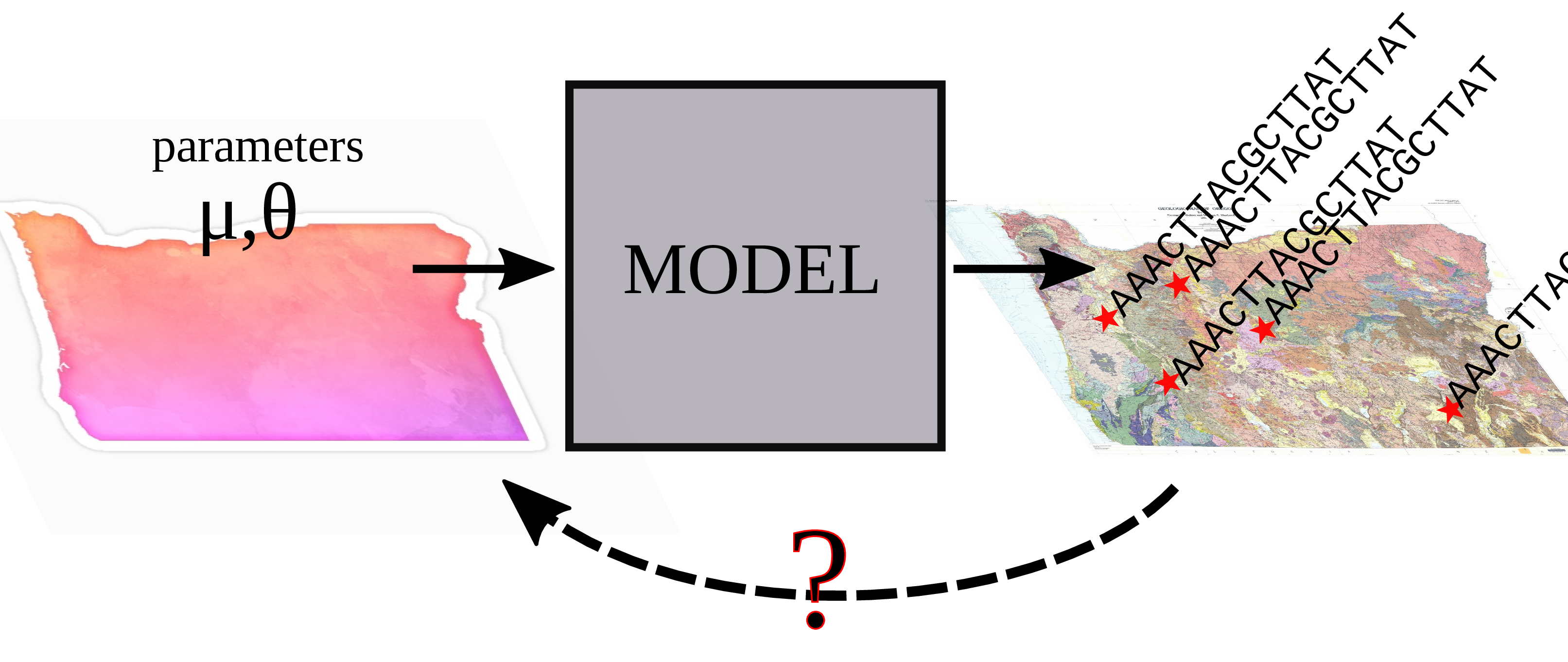
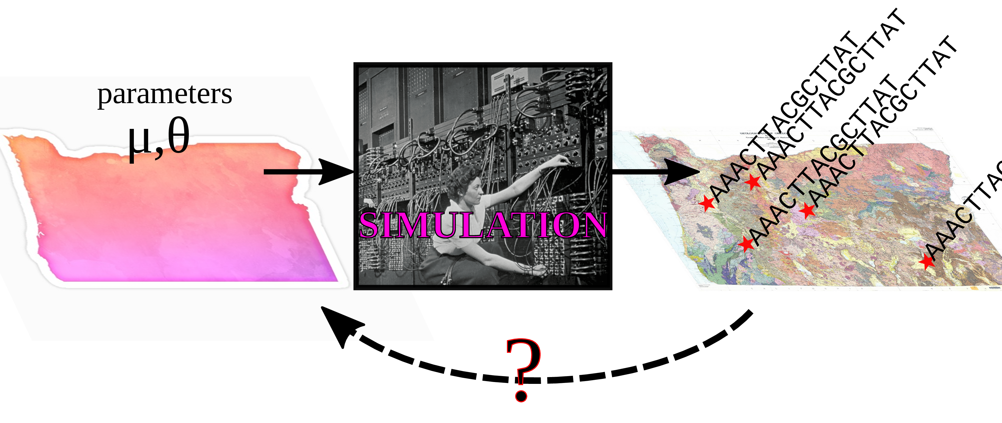
Simulation-based inference
- bespoke confirmatory simulations
- optimization of one or two parameters
- Approximate Bayesian Computation (ABC)
- deep learning
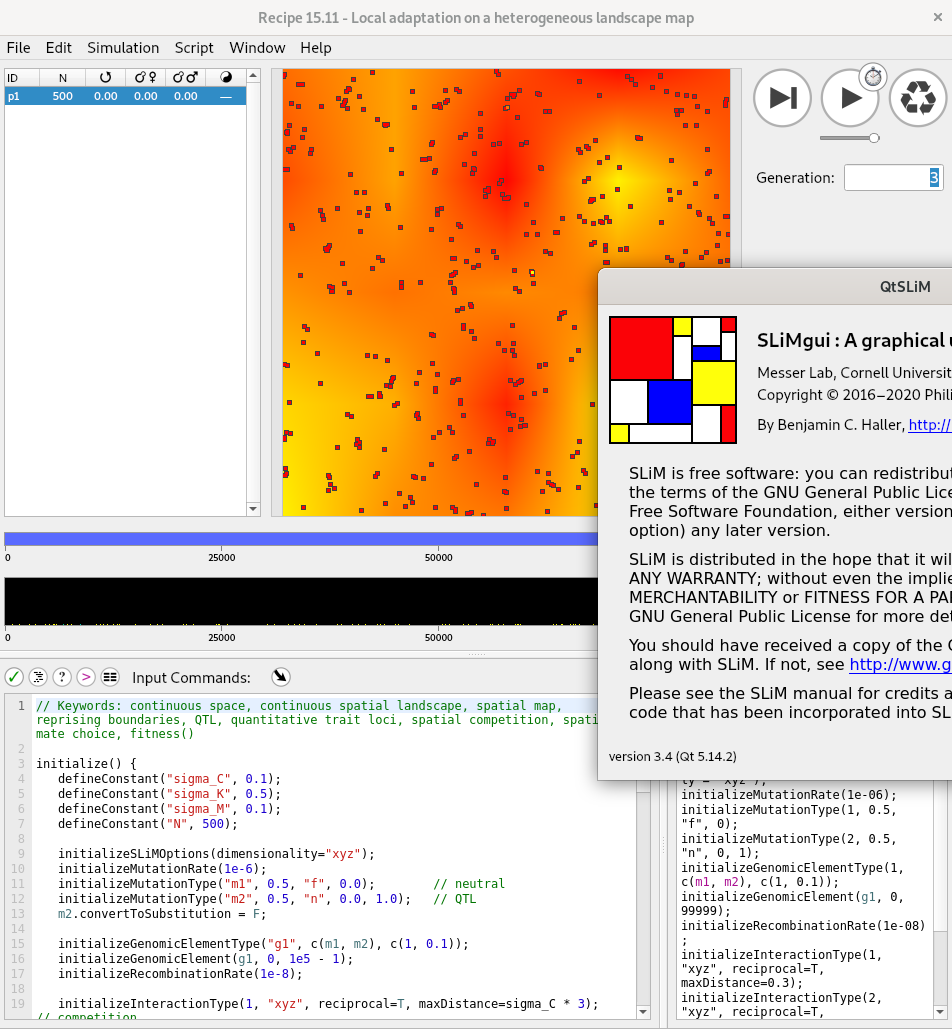
Enter SLiM
by Ben Haller and Philipp Messer
an individual-based, scriptable forwards simulator


History is a sequence of trees
For a set of sampled chromosomes, at each position along the genome there is a genealogical tree that says how they are related.

The succinct tree sequence
is a way to succinctly describe this, er, sequence of trees
and the resulting genome sequences.

jerome kelleher
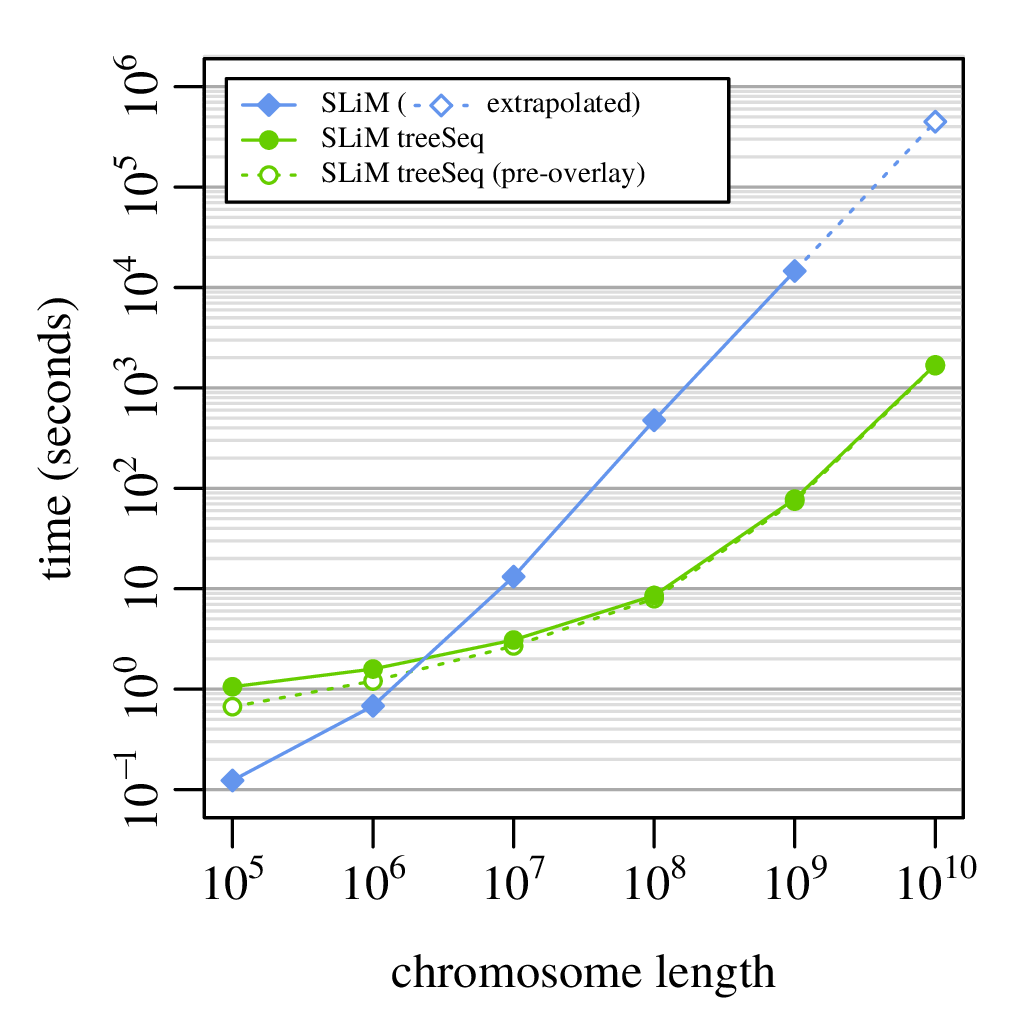
How’s it work? File sizes:
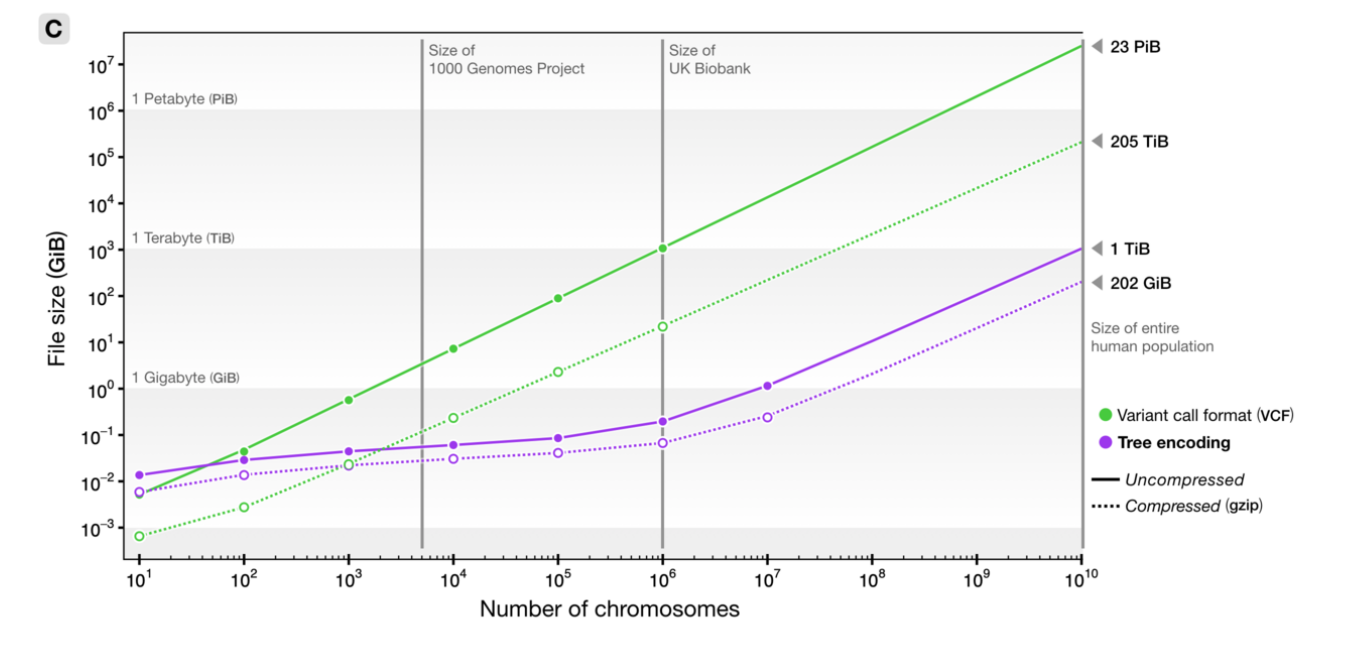
100Mb chromosomes; from Kelleher et al 2018, Inferring whole-genome histories in large population datasets, Nature Genetics


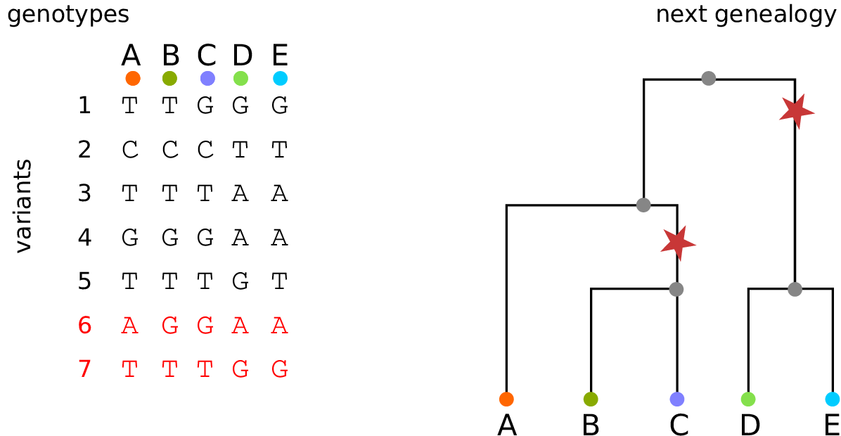
For \(N\) samples genotyped at \(M\) sites
Genotype matrix:
\(N \times M\) things.
Tree sequence:
- \(2N-2\) edges for the first tree
- \(\sim 4\) edges per each of \(T\) trees
- \(M\) mutations
\(O(N + T + M)\) things
How’s it work, 2? Computation time:
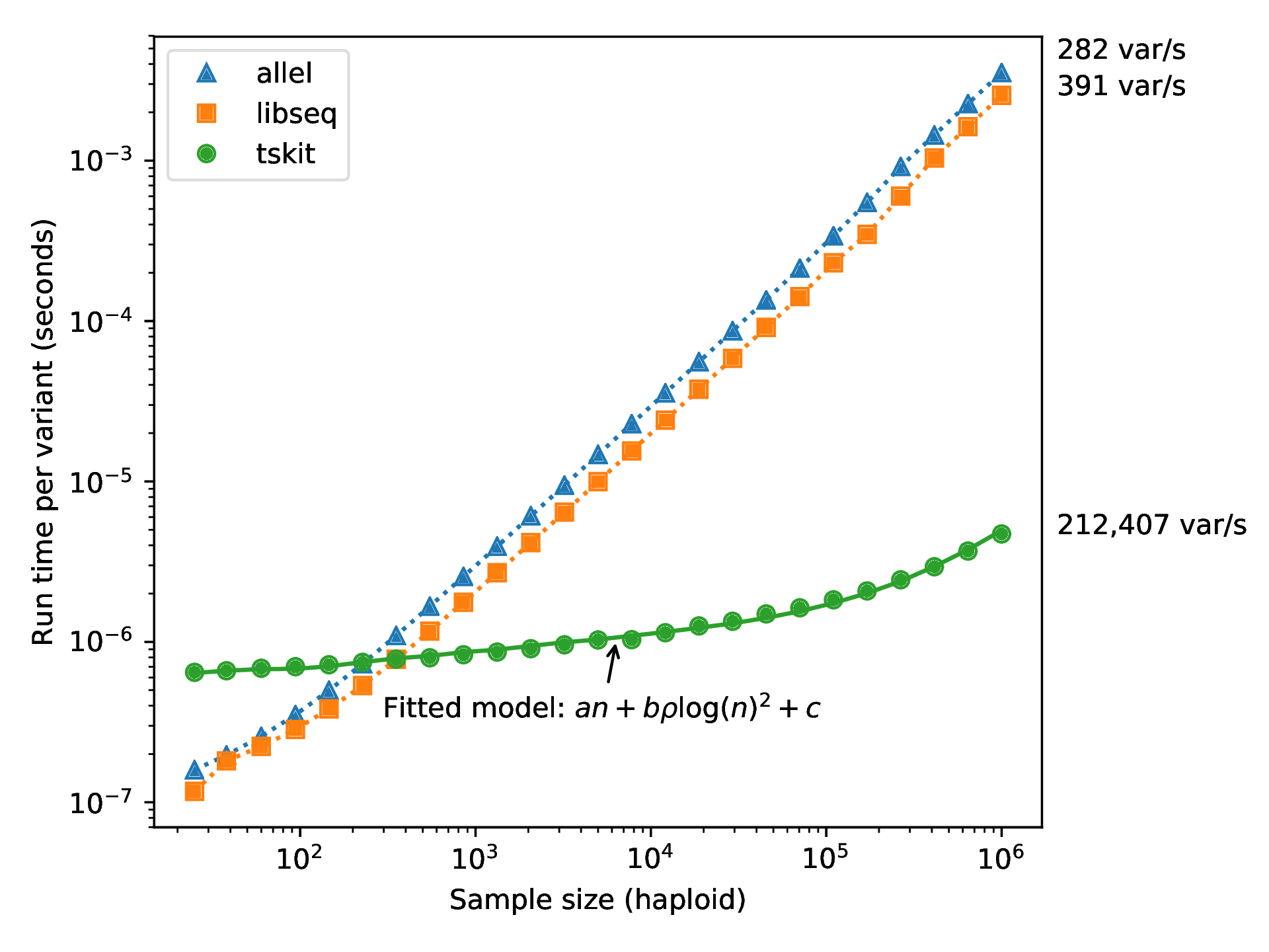
This means recording the entire genetic history of everyone in the population, ever.
It is not clear this is a good idea.
But, with a few tricks…
From Kelleher, Thornton, Ashander, and R. 2018, Efficient pedigree recording for fast population genetics simulation.
and Haller, Galloway, Kelleher, Messer, and R. 2018, Tree‐sequence recording in SLiM opens new horizons for forward‐time simulation of whole genomes


A 100x speedup!
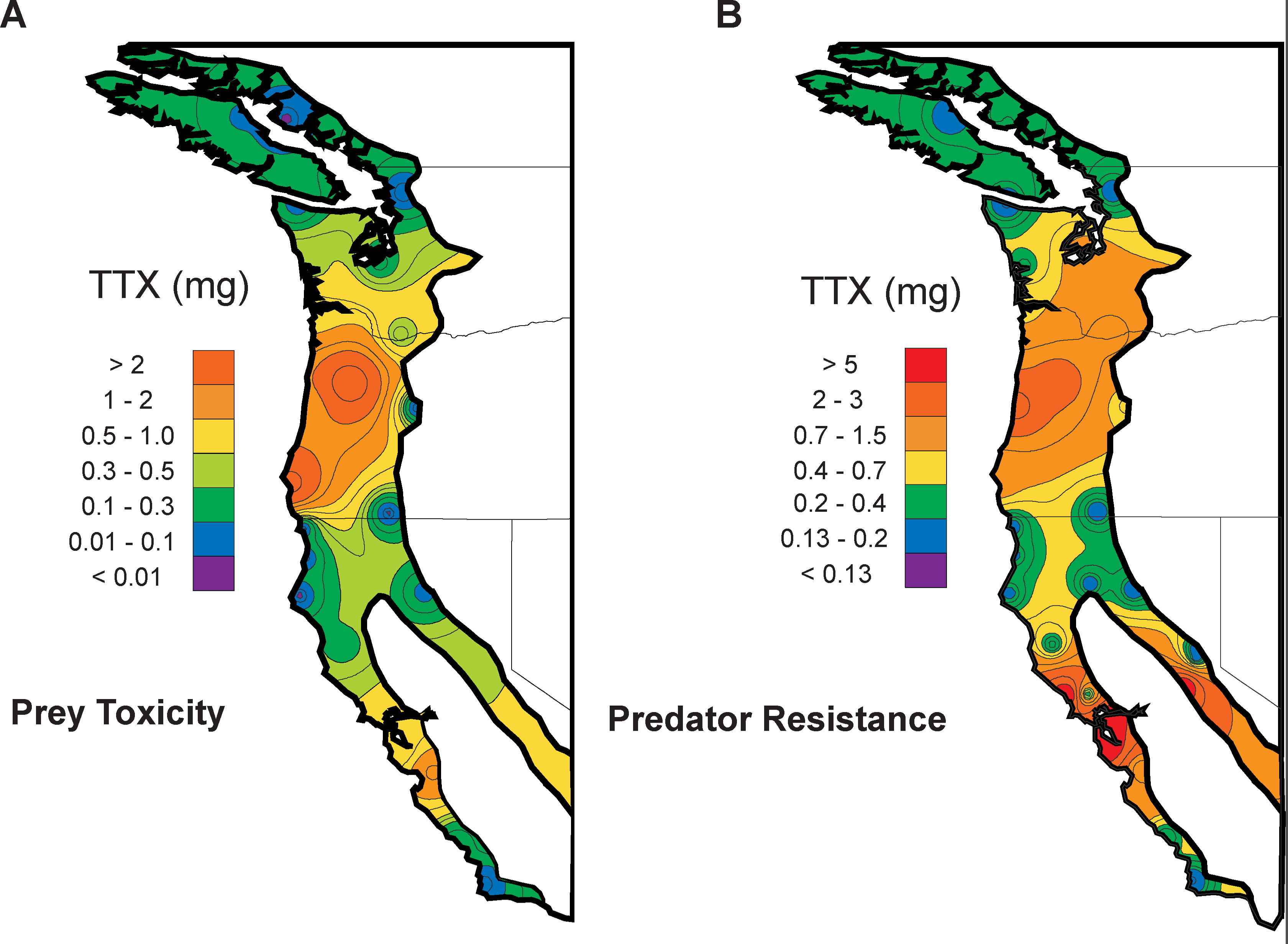
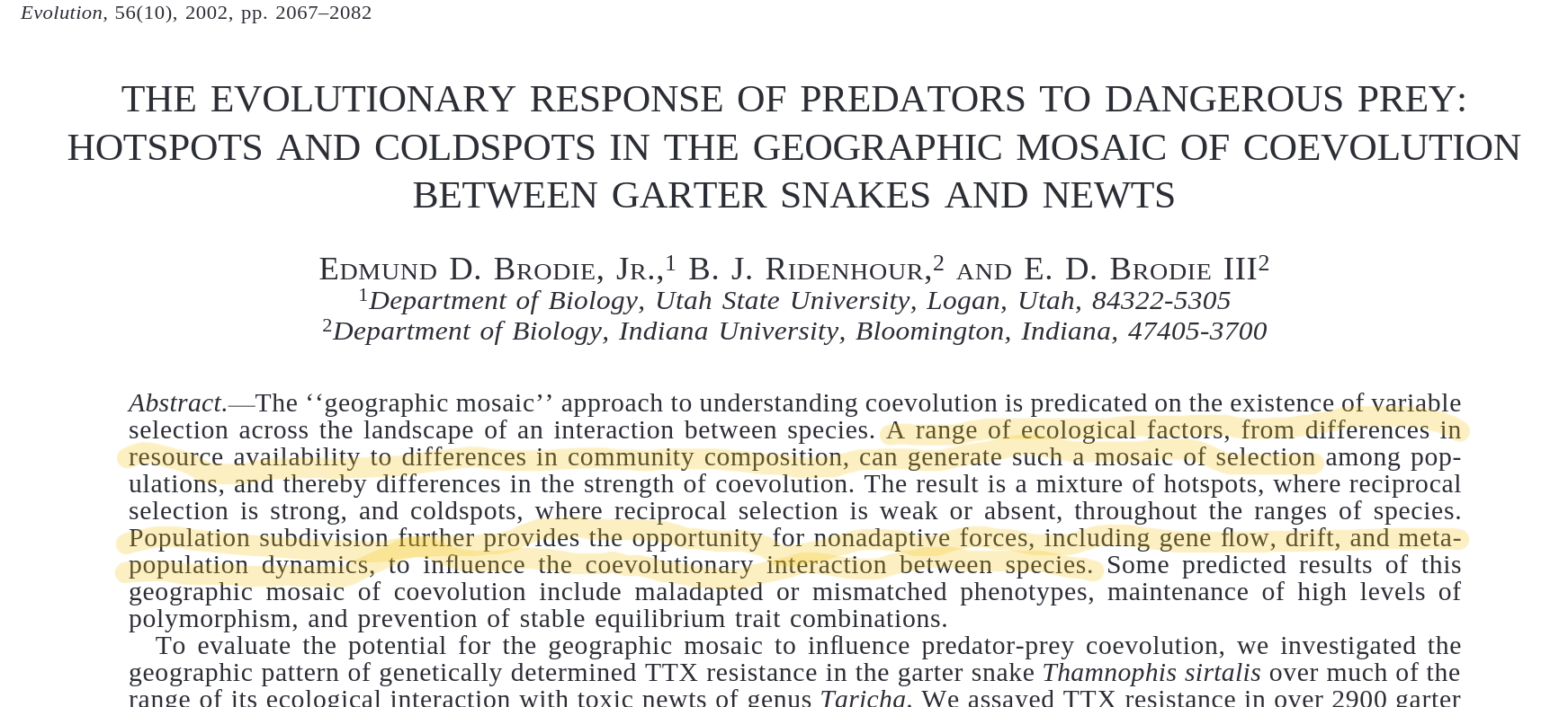
Spatial coevolution: snakes and newts

Victoria Caudill
Image from evolution.berkeley.edu
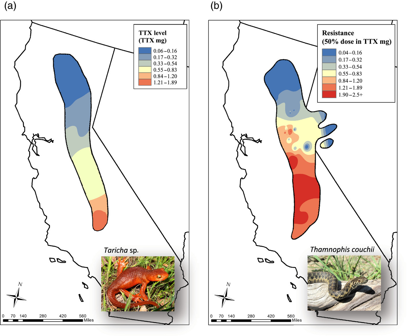
Why, and how?
A spatial co-evolutionary simulation
continuous space
local density-dependent mortality
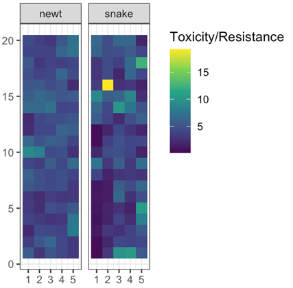
additive, costly traits (“toxicity” and “resistance”)
various genetic architectures
snakes may encounter nearby newts, outcome depends on difference in traits:
- snake eats newt, gets fitness benefit, or
- snake dies, newt escapes
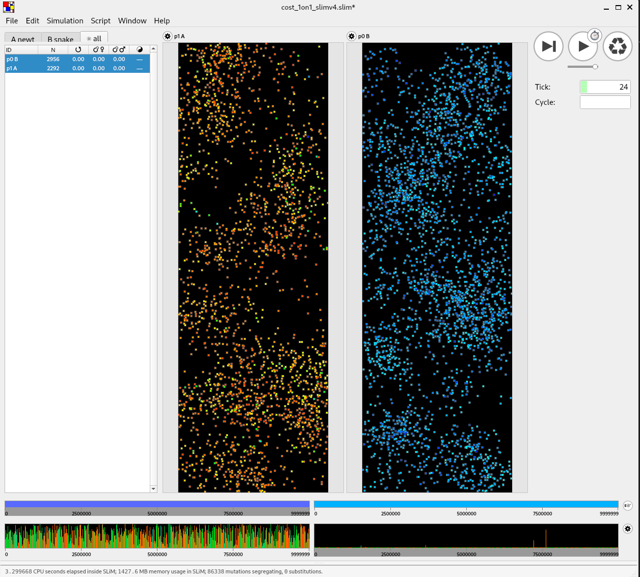
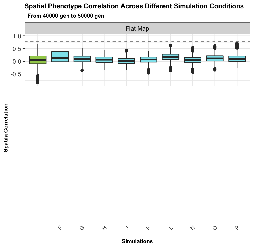
No spatial correlation on a flat map
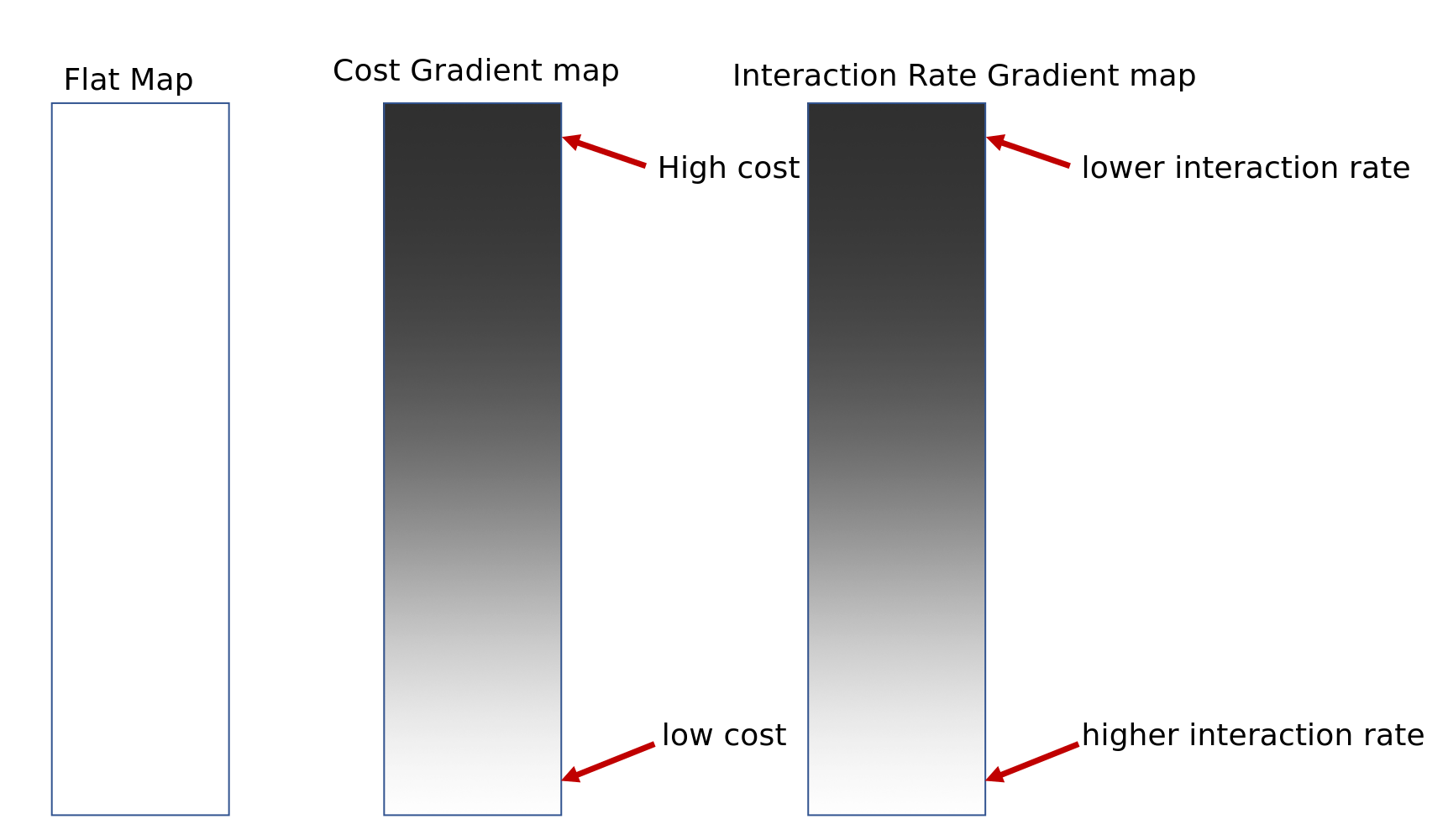
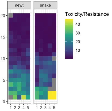
Add some heterogeneity
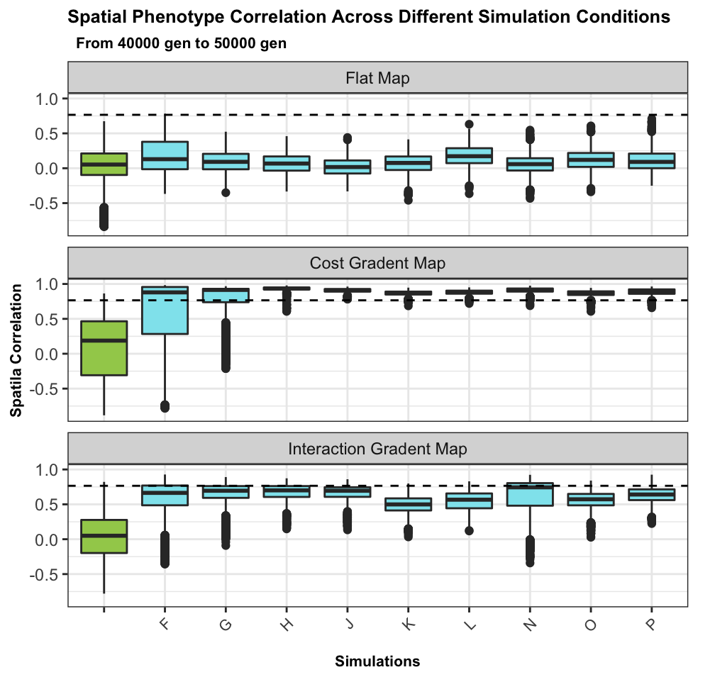
Conclusions
such large correlated differences across the landscape unlikely to be due to nonadaptive forces
spatial heterogeneity in ecological factors much more plausible
trait genetic architecture has little effect, given sufficient variation
Victoria Caudill
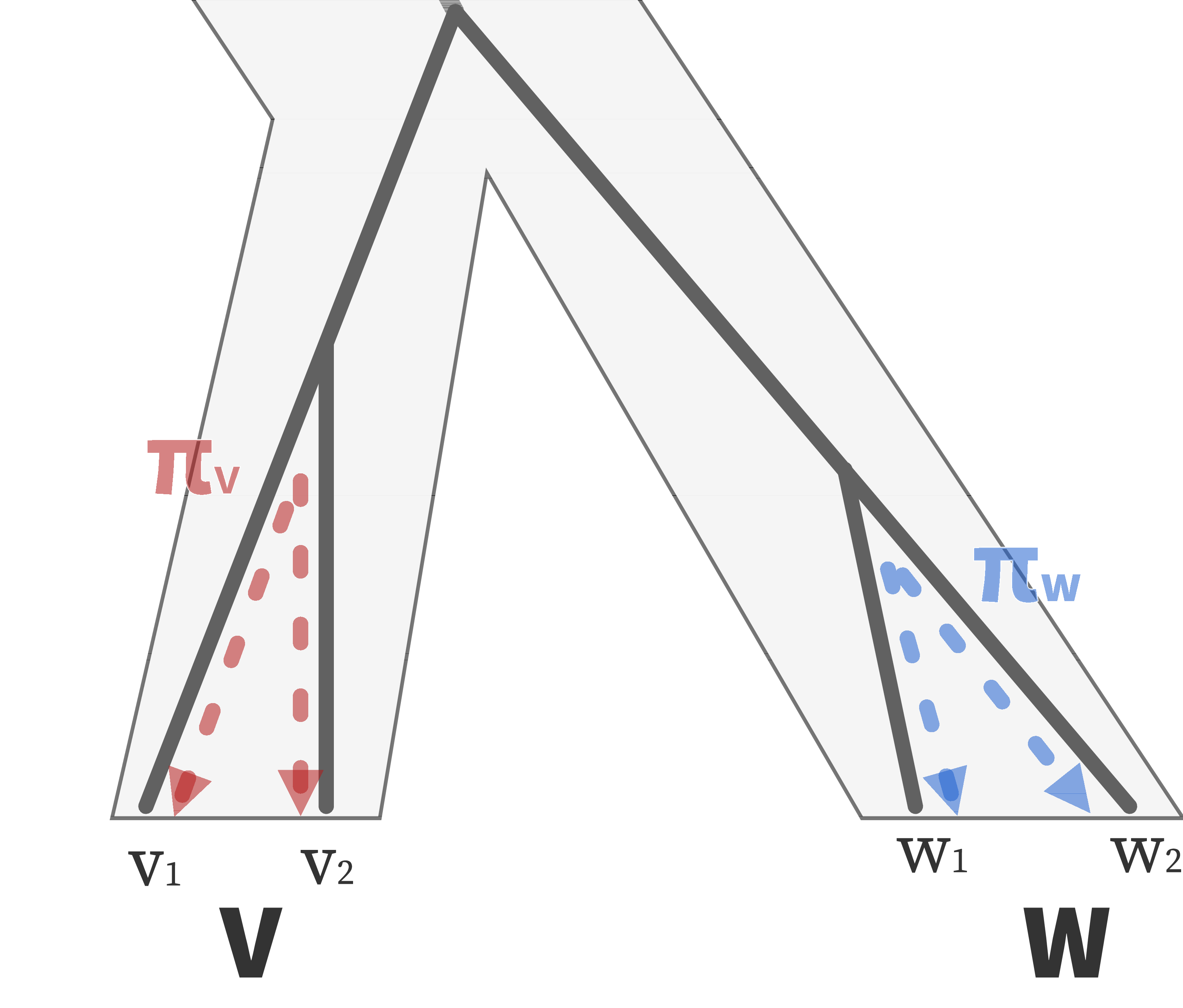
Landscapes of genetic diversity


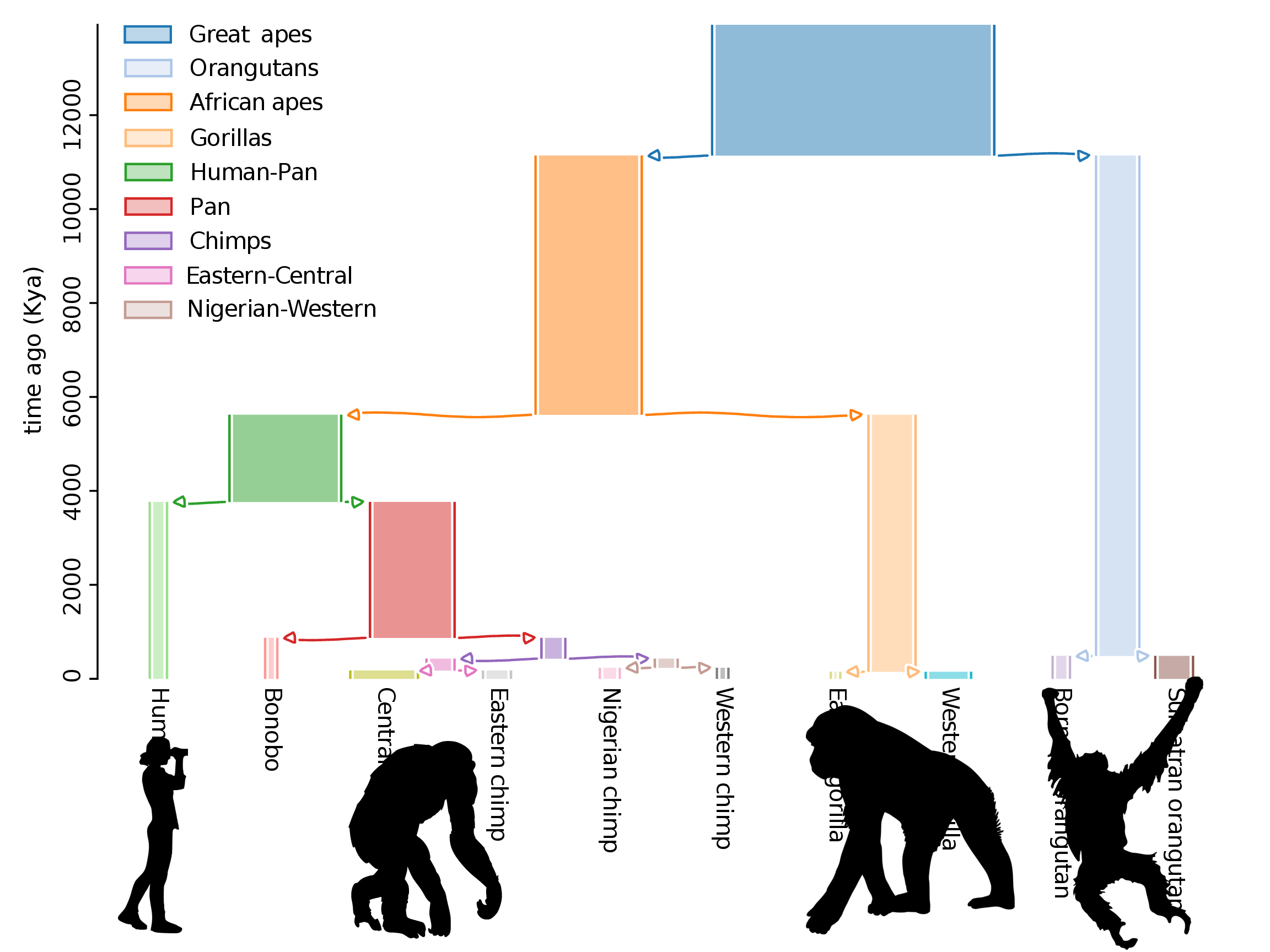
Landscapes of genetic diversity within groups of species
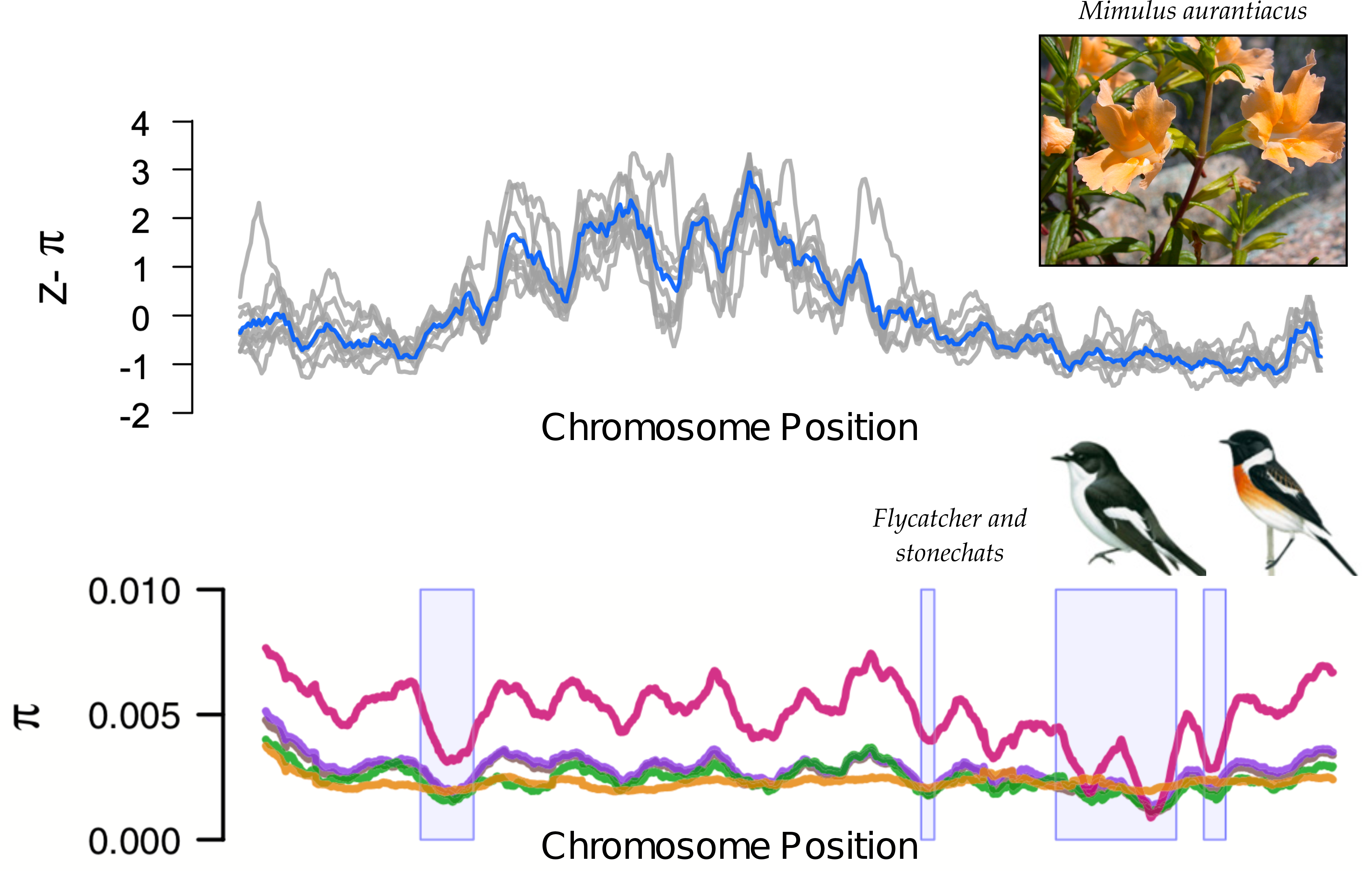
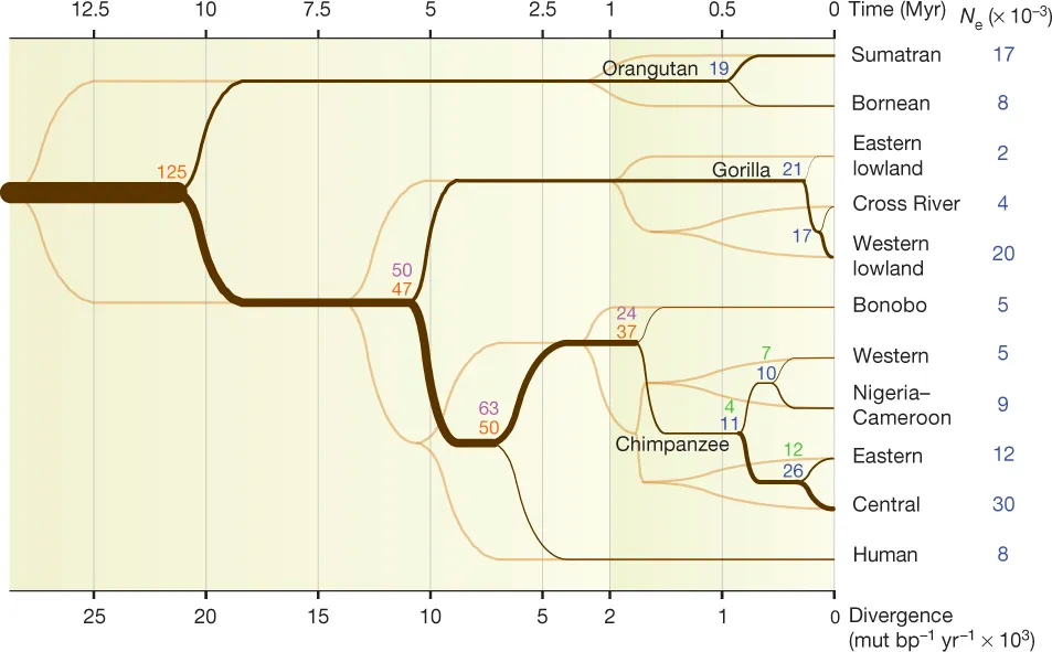
The study system: “us”
- High quality genomic data for 5 species
- Deep divergence, spanning ~60N generations
- Conservation of genes, recombination rate and other genomic features
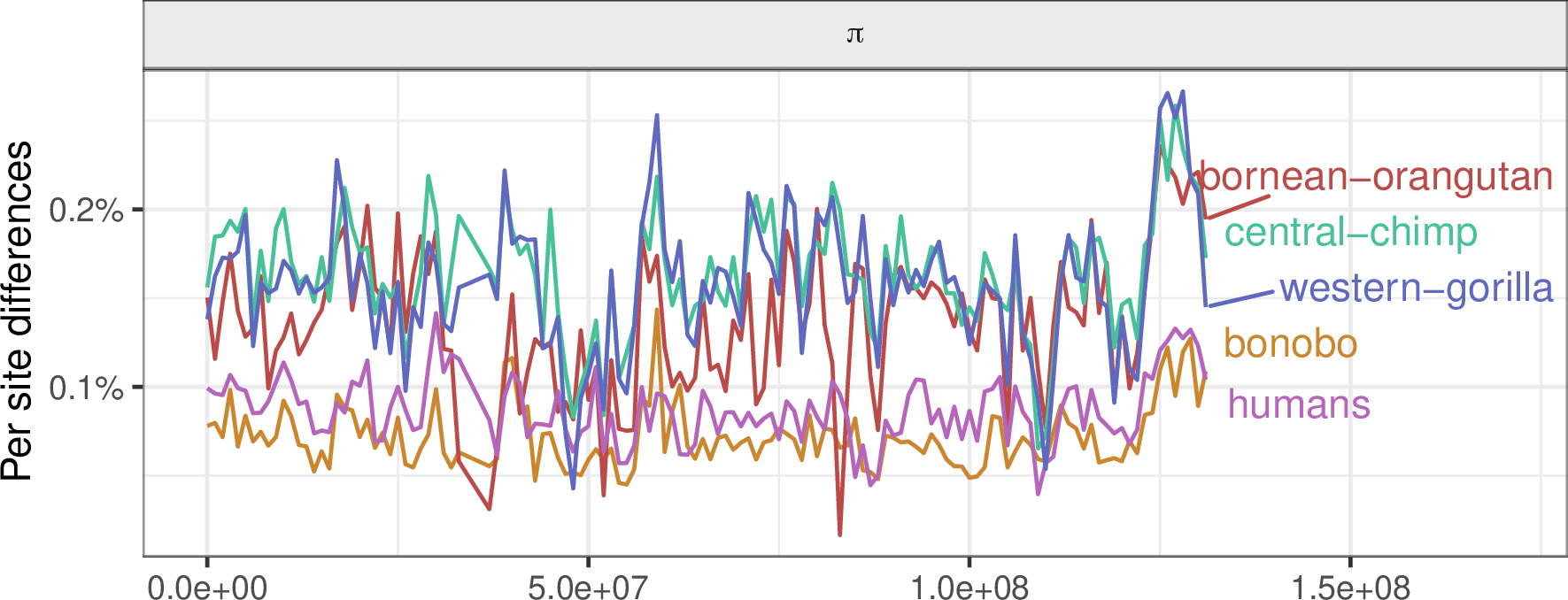
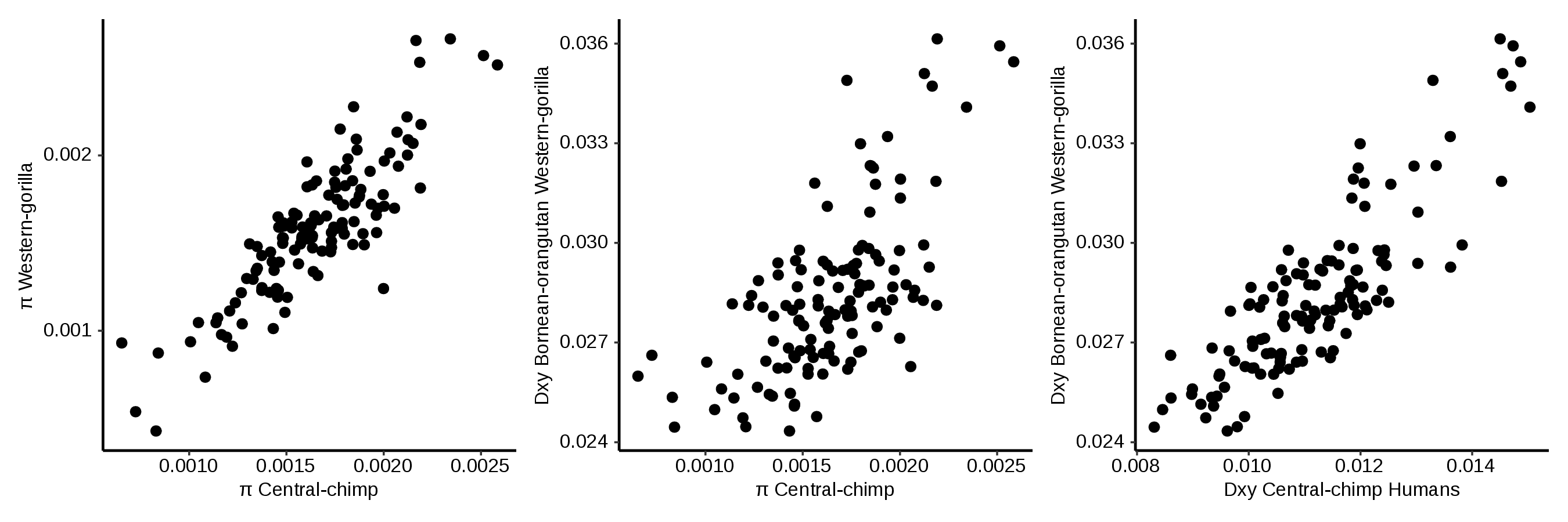
Genetic diversity in the great apes: chromosome 12
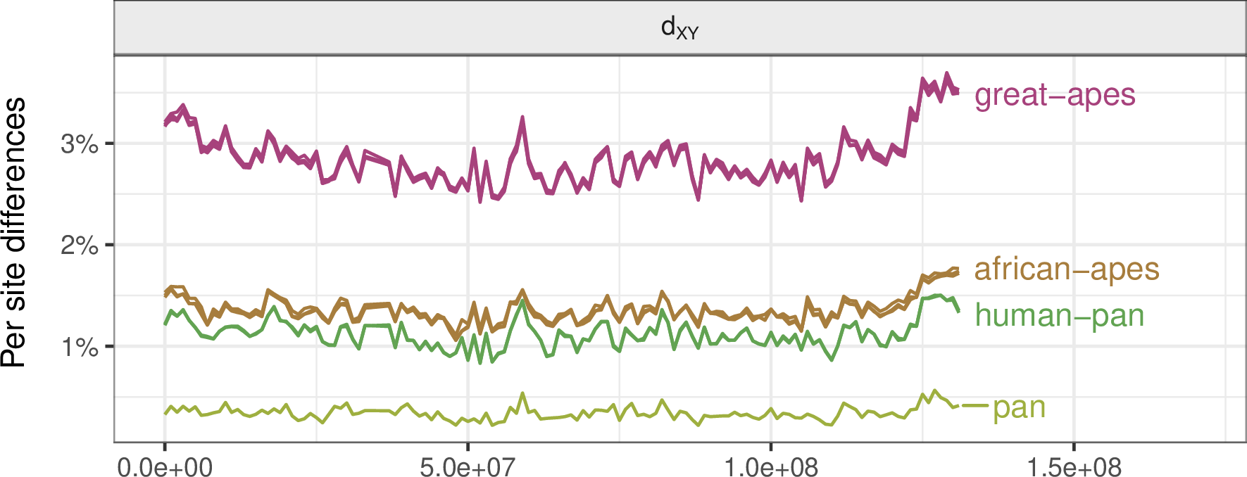
Genetic divergence between the great apes: chromosome 12
Goals
- How correlated are landscapes for closely related species?
- How much is due to shared footprints of
- history?
- selection? what kind?
- mutational processes?
linked selection: The indirect effects of selection on genomic locations that are linked to the sites under selection by a lack of recombination.
Selection tends to decrease diversity, over a distance determined by recombination rate.
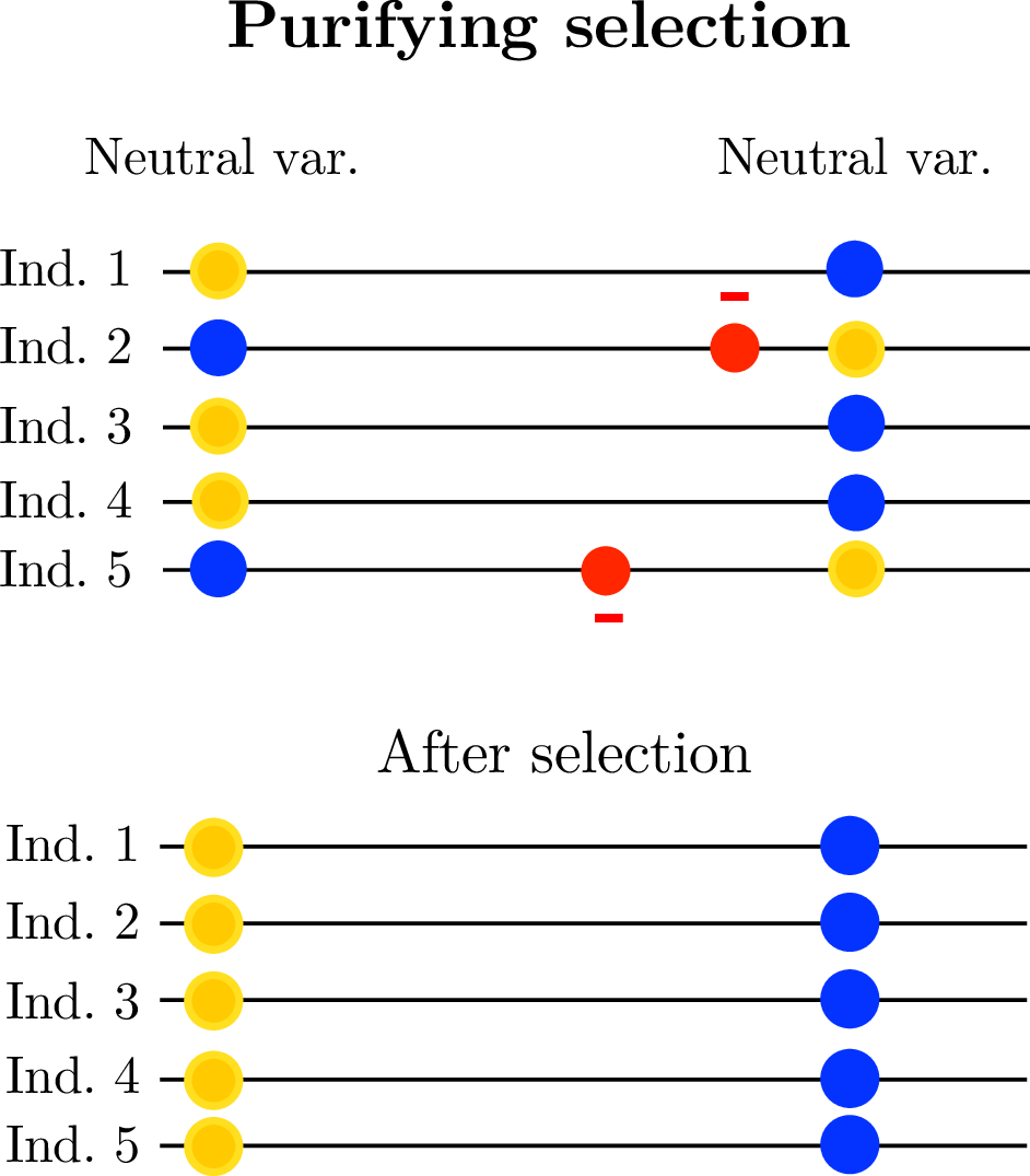
Diversity correlates with recombination rate
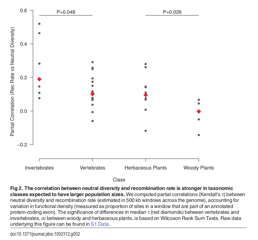
Hudson 1994; Cutter & Payseur 2013; Corbett-Detig et al 2015
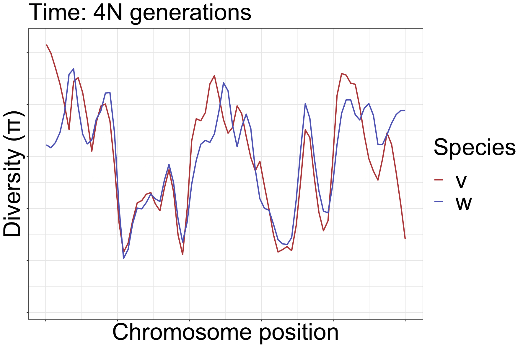
How diversity landscapes change
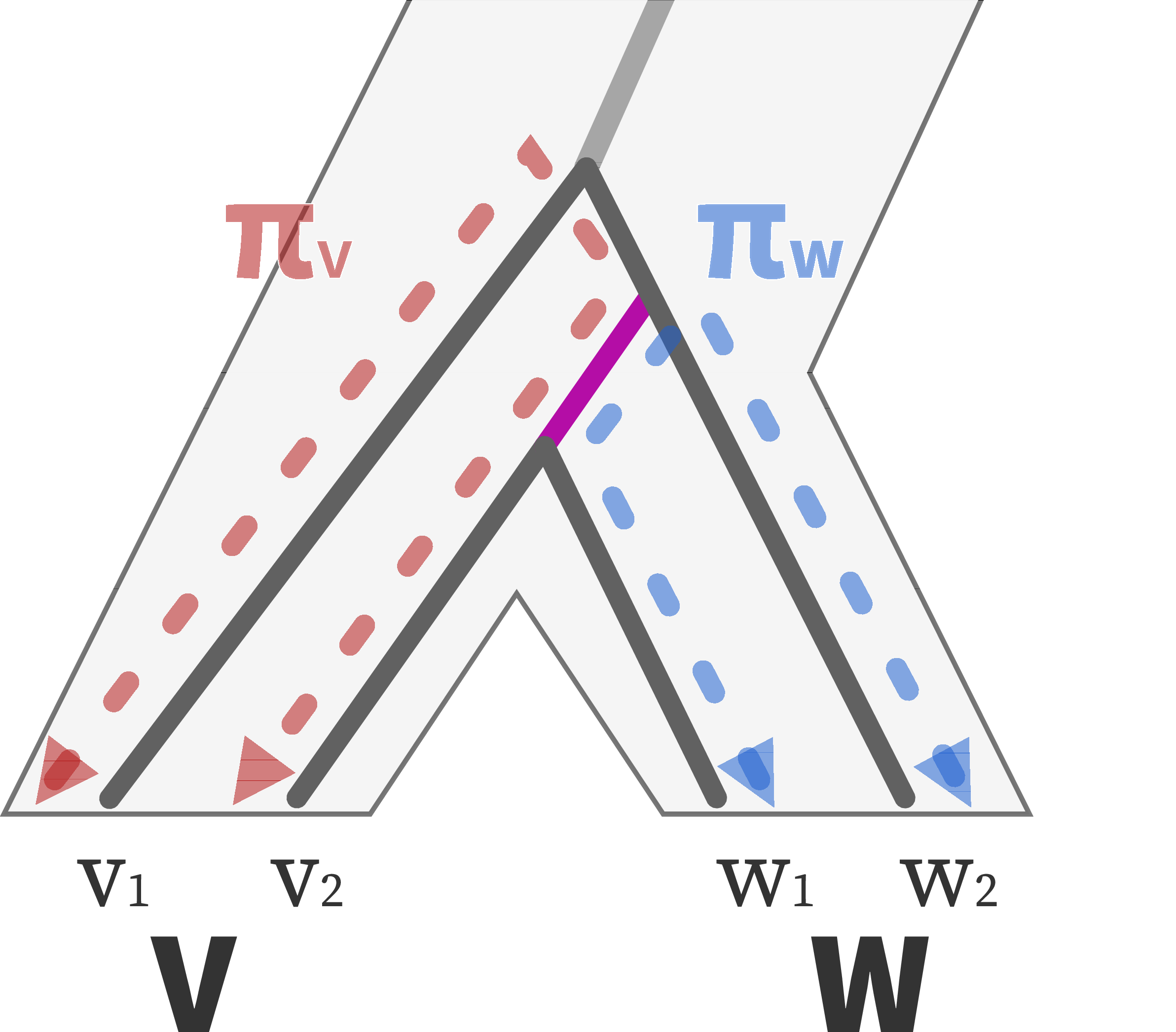
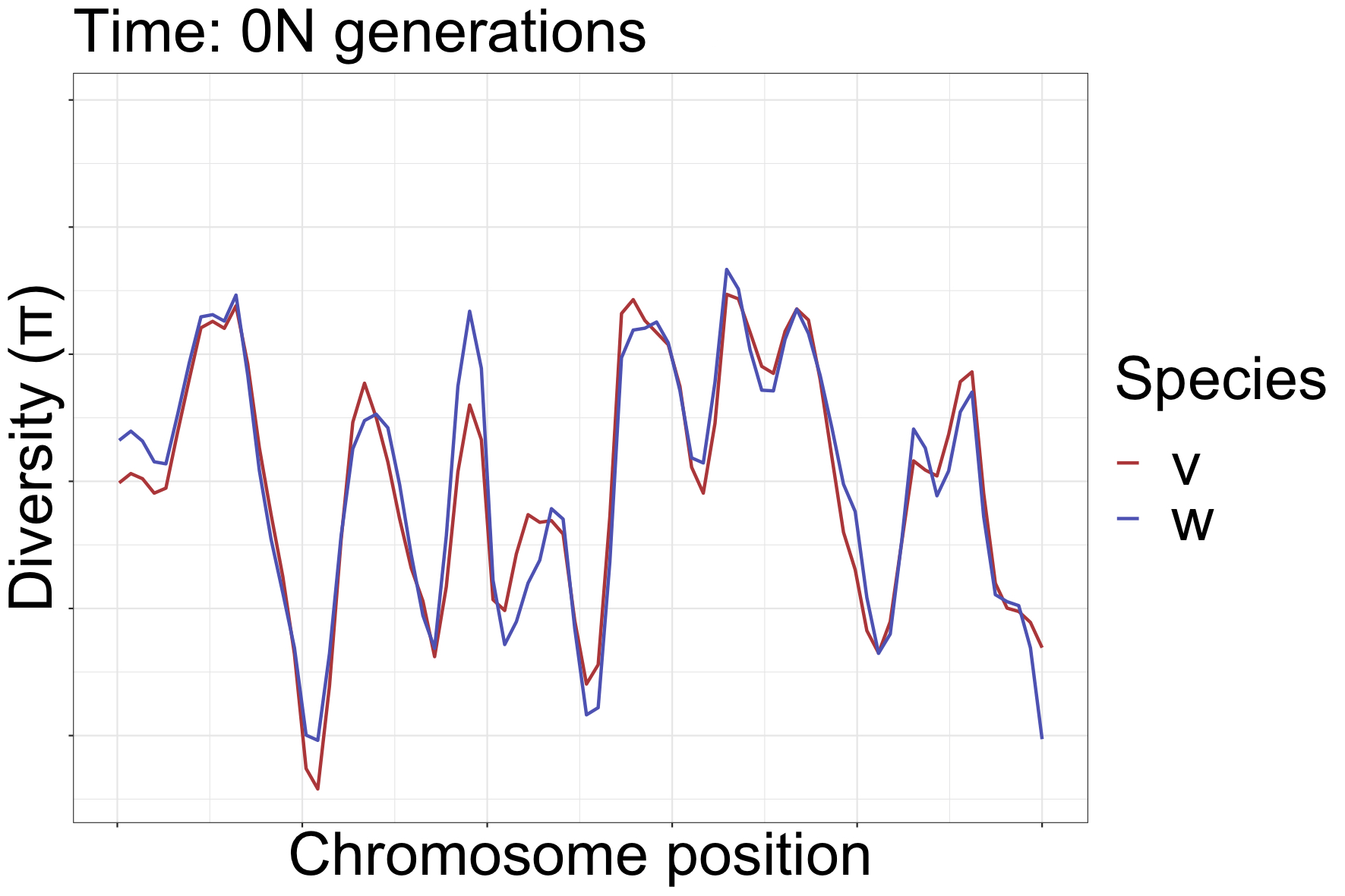
How diversity landscapes change

How diversity landscapes change
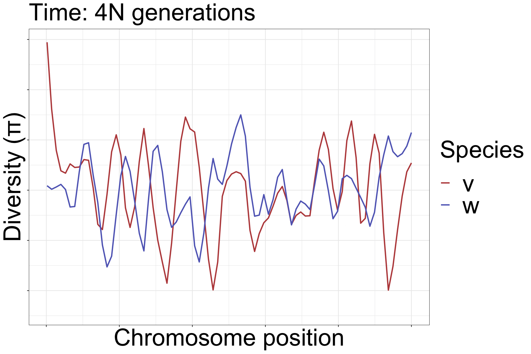
How can landscapes stay correlated?
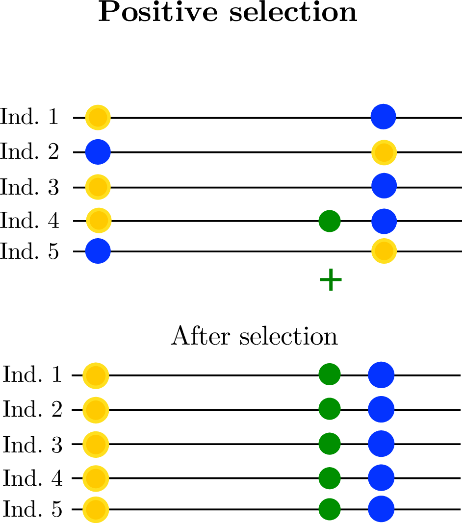
- shared processes:
- positive, negative selection
- mutation rate variation
- GC-biased gene conversion

How can landscapes stay correlated?
- shared processes:
- positive, negative selection
- mutation rate variation
- GC-biased gene conversion
How can landscapes stay correlated?
- shared processes:
- positive, negative selection
- mutation rate variation
- GC-biased gene conversion
SLiMulations
.jpg)
Back to the data

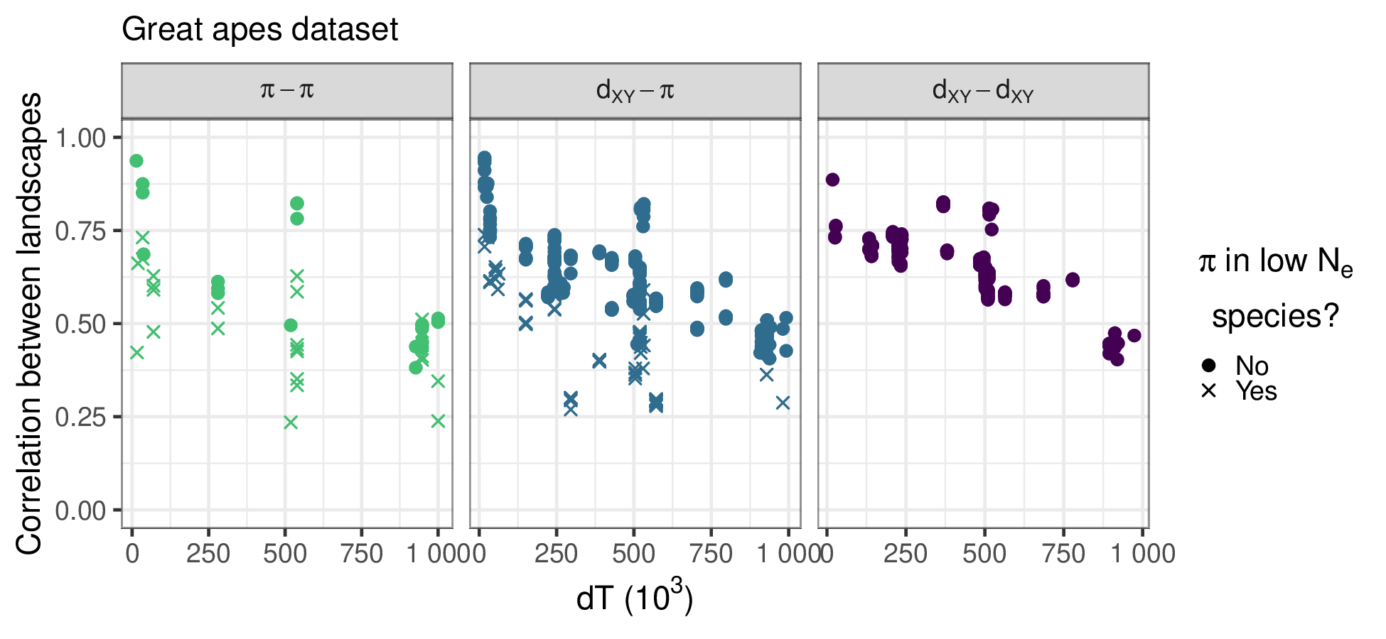
The data: empirical correlations for chromosome 12 in the great apes
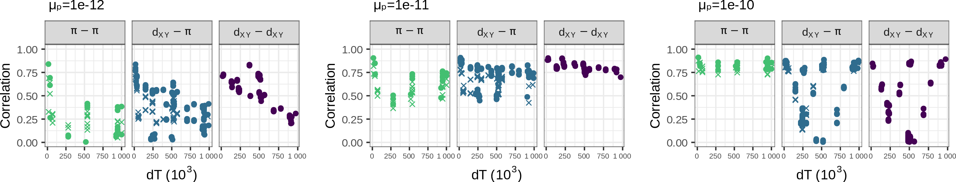
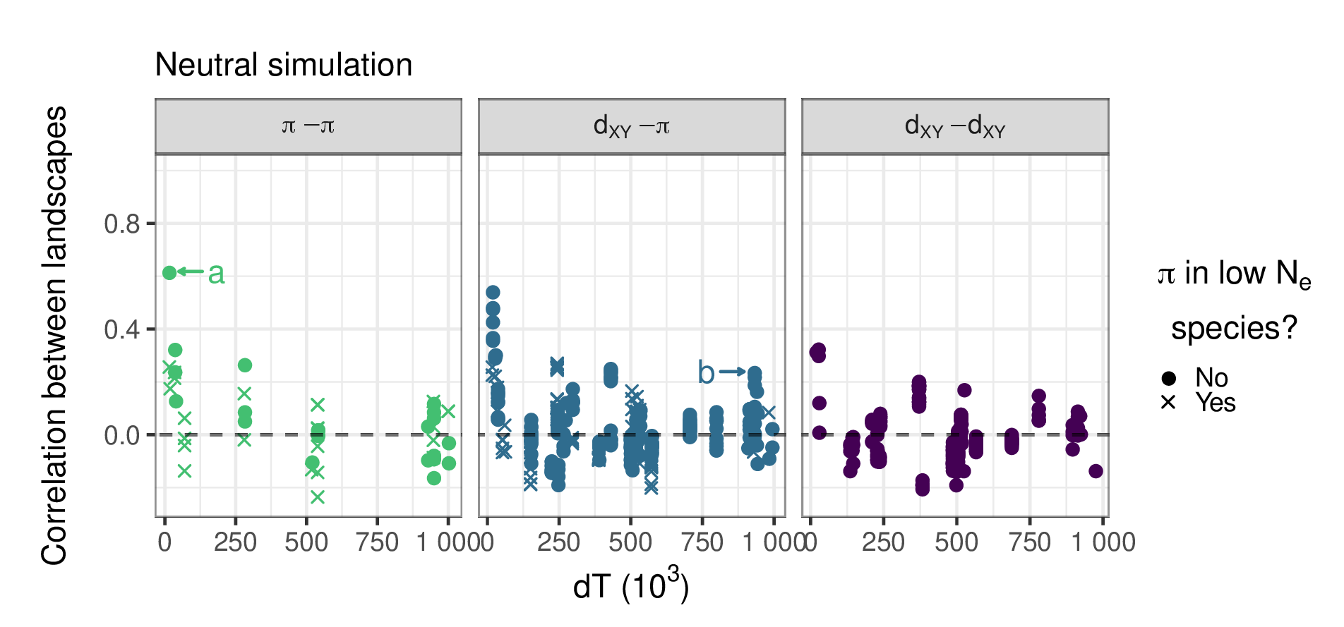
No correlation under neutrality
- correlations decay to zero quickly with split time
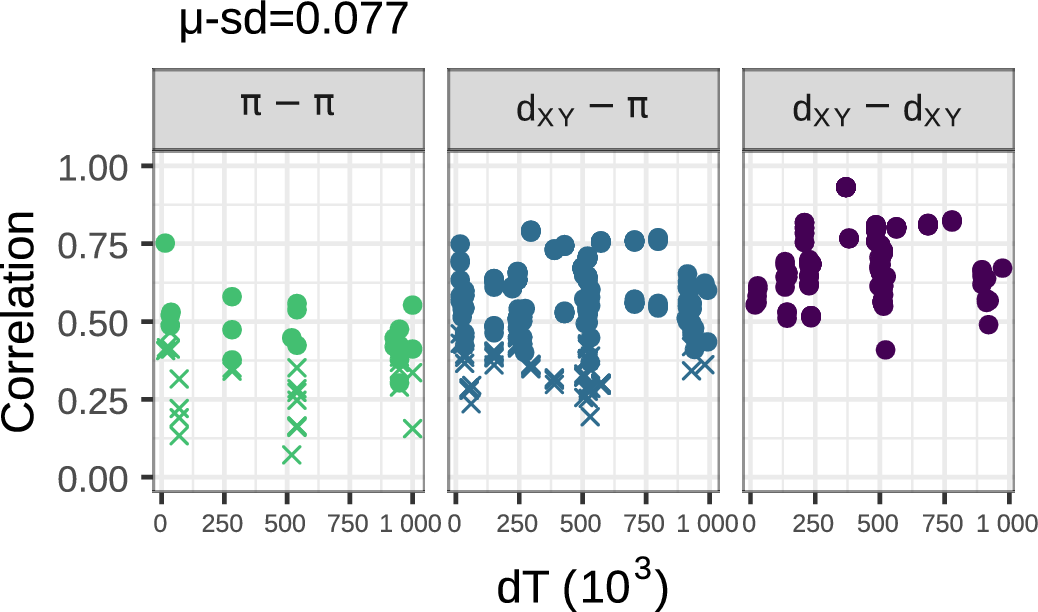
Mutation rate variation can contribute
- but correlations do not decay with time
Negative selection produces weak correlations
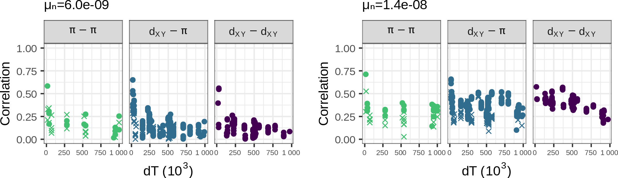
Positive selection produces strong correlations
- sometimes too strong
\[ \vphantom{ d_{xy} = \pi_\text{anc} \nearrow + \mu T_\text{MRCA} \searrow } \]
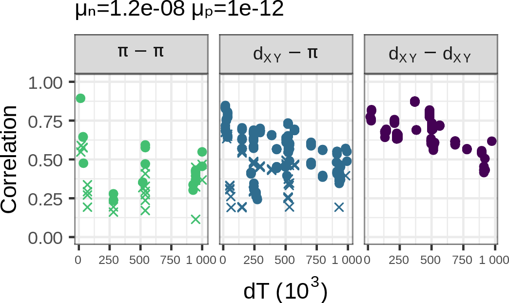
The best fit: both!
- chosen from 37 distinct simulations
- deleterious mutations: \(1.2 \times 10^{-8}\)
- beneficial mutations: \(10^{-12}\)
Conclusions
- positive selection most necessary for a good fit
- best guess: \(\approx 10\%\) of fixations on human lineage due to positive selection (1/250 years);
- \(\approx\) 70% of mutations in exons deleterious
- fixation rate in exons reduced by half
- GC-biased gene conversion causes “smile” at ends of chromosomes
Software development goals
- open
- welcoming and supportive
- reproducible and well-tested
- backwards compatible
- well-documented
- capacity building

Thanks!
- Andy Kern
- Victoria Caudill
- Murillo Rodrigues
- Gilia Patterson
- Chris Smith
- Nate Pope
- Jiseon Min
- Clara Rehmann
- Bruce Edelman
- Anastasia Teterina
- Matt Lukac
- the rest of the Co-Lab
Funding:
- NIH NIGMS
- NSF DBI
- Jerome Kelleher
- Ben Haller
- Ben Jeffery
- Yan Wong
- Elsie Chevy
- Madeline Chase
- Sean Stankowski
- Matt Streisfeld
![]()
![]()
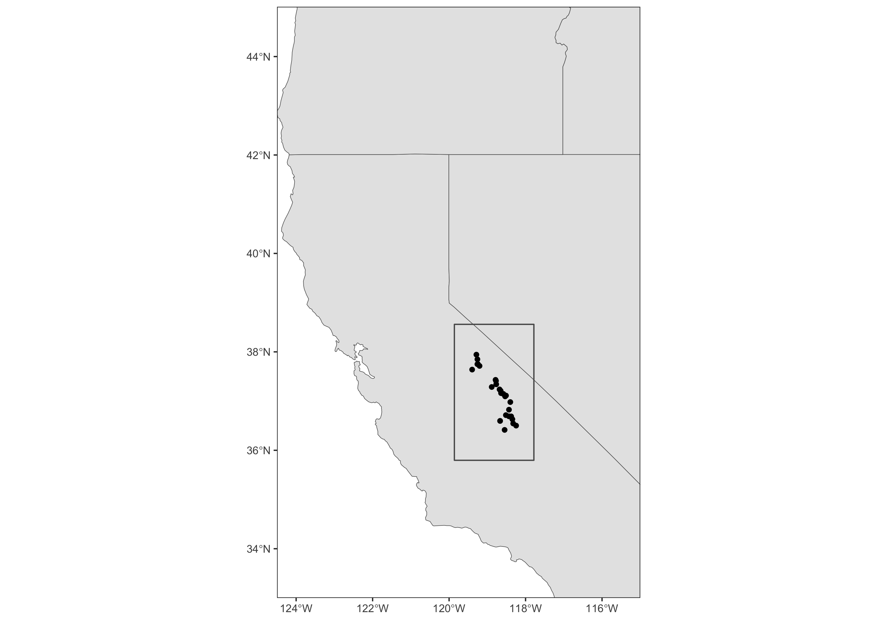
Nebria ingens/riversi
- ground beetles
- live on flowing snowmelt in the Sierra Nevada of California
- cannot fly
- live 1–2 years

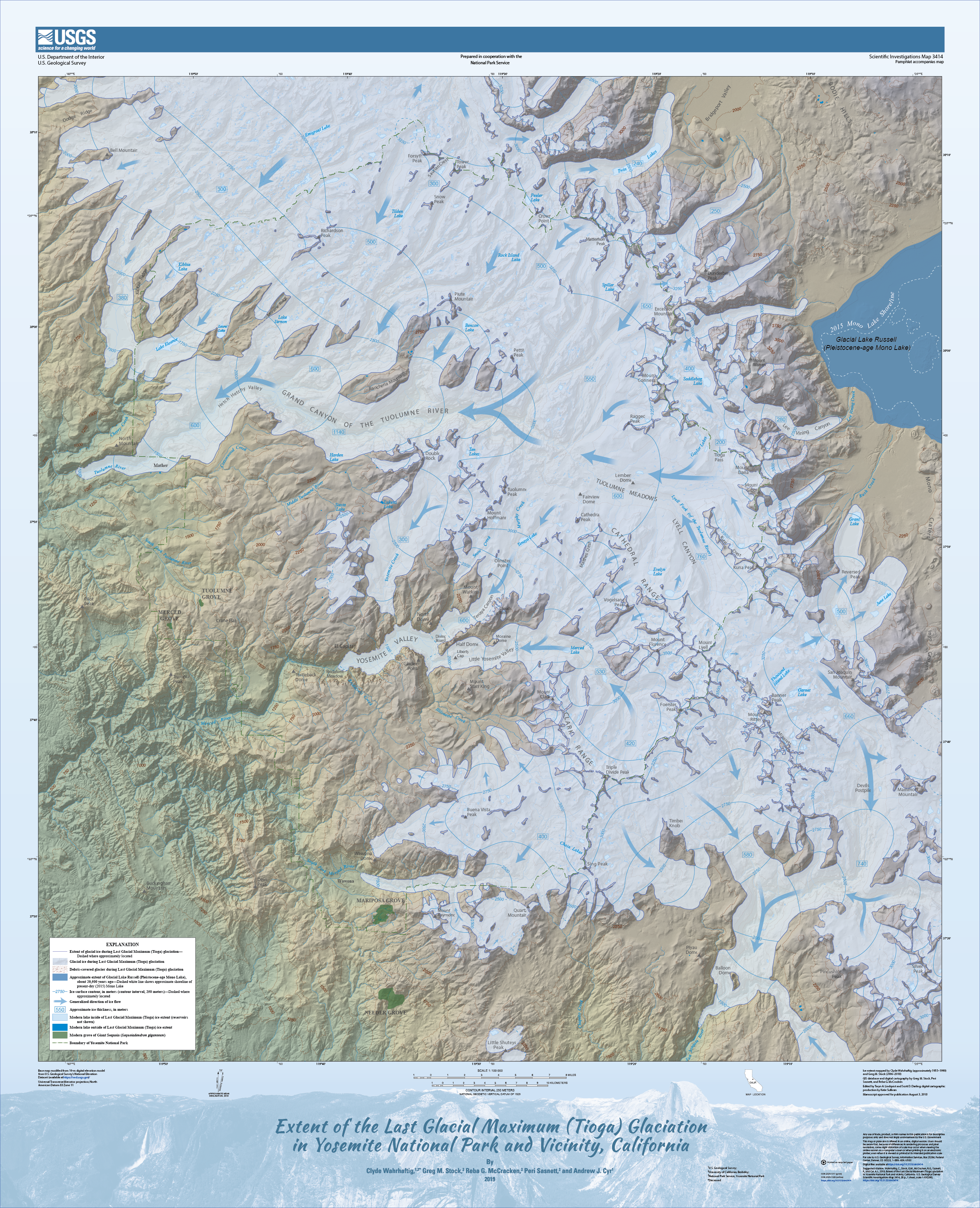
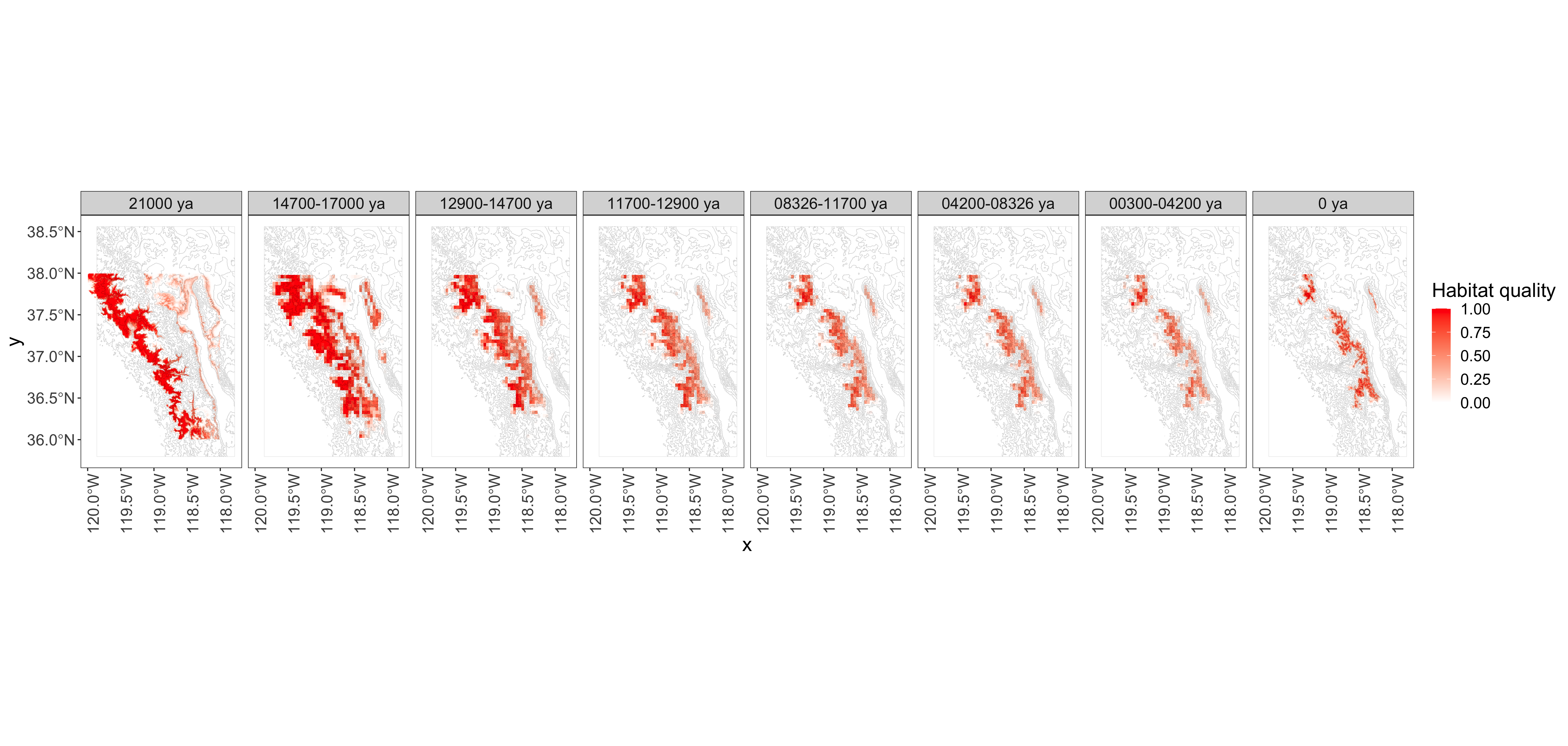
Good habitat followed the glaciers uphill (SDM by Yi-Ming Weng).
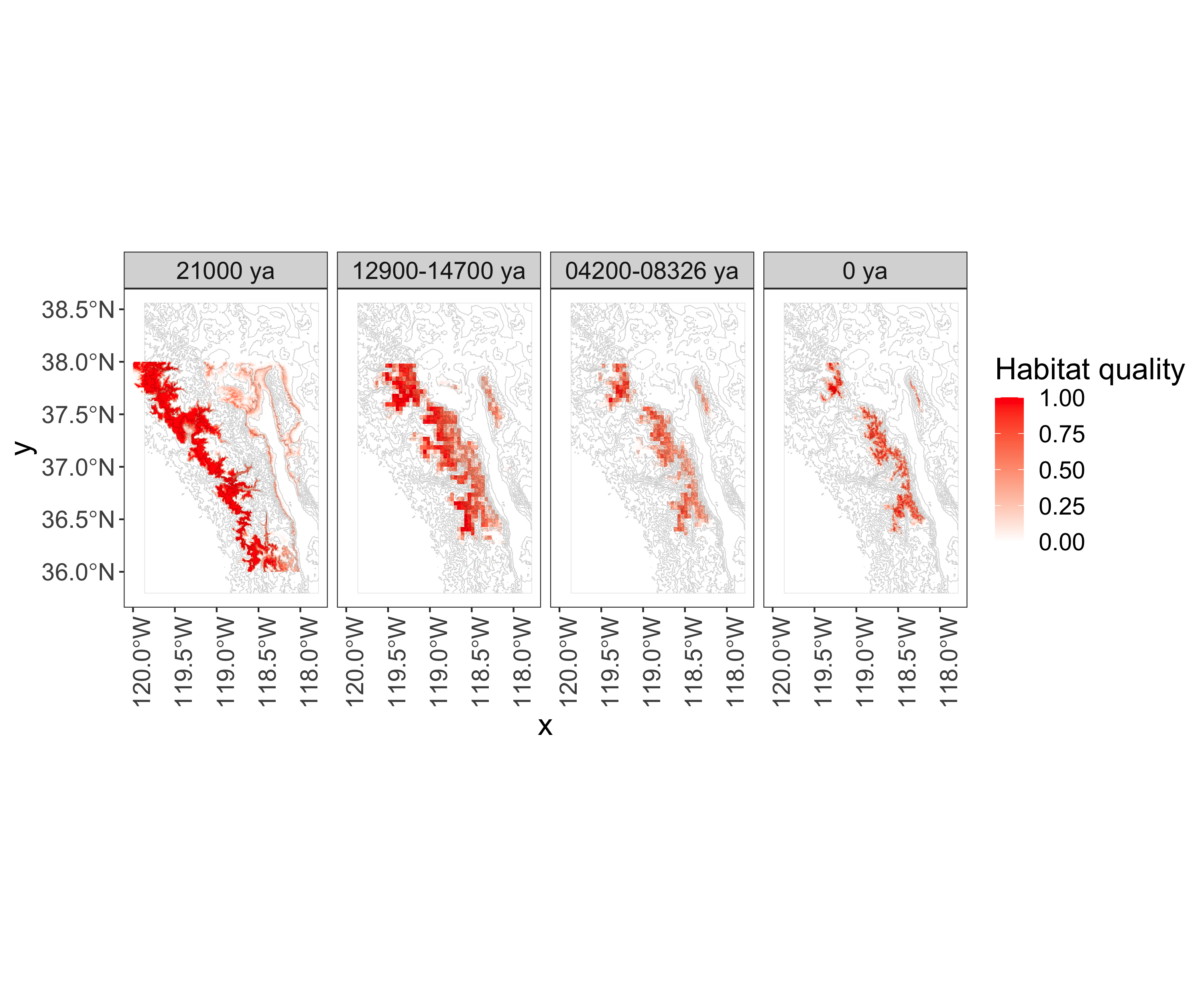
Goals
- What was the spatial demographic history of Nebria since the LGM?
- Where did the ancestors of today’s beetles live in the past?
- Were the ancestors of N. ingens and N. riversi distinct at the LGM?
Data
Collected by Yi-Ming Weng and Sean Schoville:
- 384 beetles at 27 sites
- low coverage WGS
- some presence/absence data
- expert knowledge about good locations
- a species distribution model